Scraping the Daily India Covid-19 Tracker for CSV Data

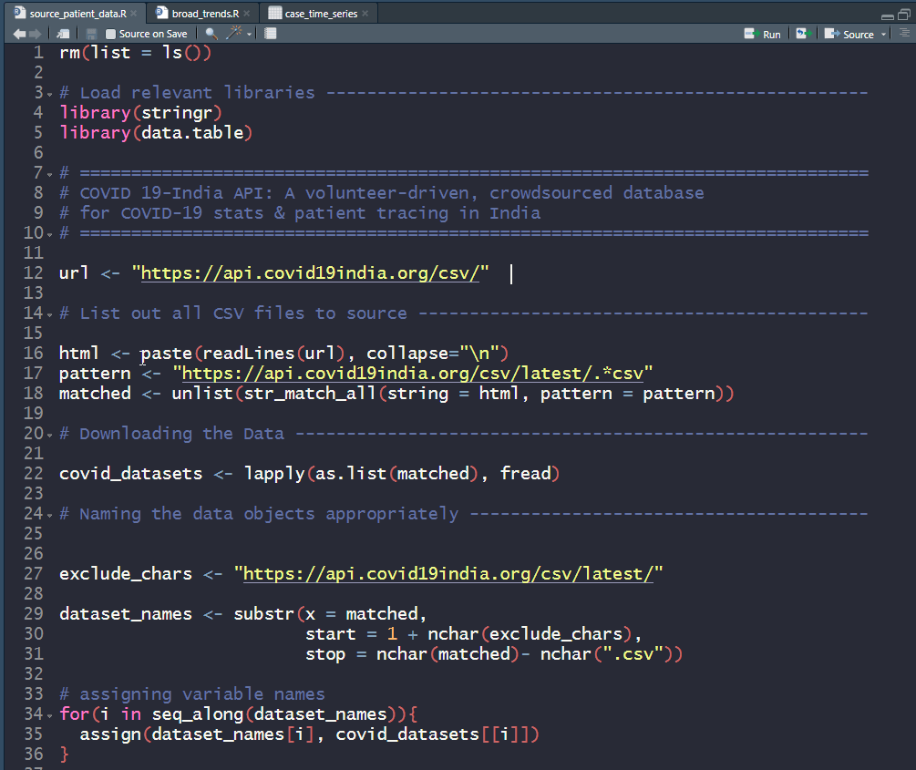
This is a very short post that will be very useful to help you quickly set up your COVID-19 datasets. I’m sharing code at the end of this post that scrapes through all CSV datasets made available by COVID19-India API.

Copy paste this standalone script into your R environment and get going!

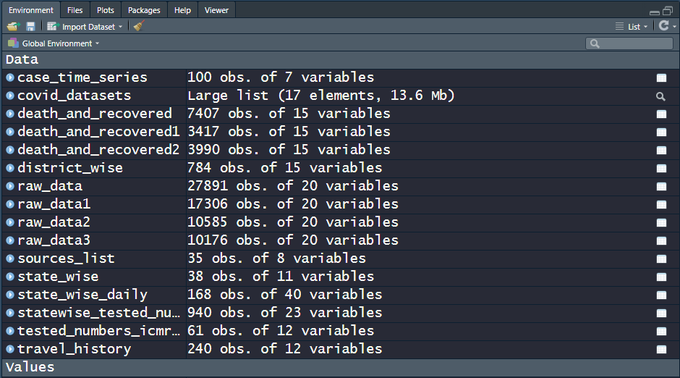
There are 15+ CSV files on the India COVID-19 API website. raw_data3 is actually a live dataset and more can be expected in the days to come, which is why a script that automates the data sourcing comes in handy.  Snapshot of the file names and the data dimensions as of today, 100 days since the first case was recorded in the state of Kerala —

Image

My own analysis of the data and predictions are work-in-progress, going into a Github repo. Execute the code below and get started analyzing the data and fighting COVID-19!

rm(list = ls())
# Load relevant libraries -----------------------------------------------------
library(stringr)
library(data.table)
# =============================================================================
# COVID 19-India API: A volunteer-driven, crowdsourced database
# for COVID-19 stats & patient tracing in India
# =============================================================================
url <- "https://api.covid19india.org/csv/"
# List out all CSV files to source --------------------------------------------
html <- paste(readLines(url), collapse="\n")
pattern <- "https://api.covid19india.org/csv/latest/.*csv"
matched <- unlist(str_match_all(string = html, pattern = pattern))
# Downloading the Data --------------------------------------------------------
covid_datasets <- lapply(as.list(matched), fread)
# Naming the data objects appropriately ---------------------------------------
exclude_chars <- "https://api.covid19india.org/csv/latest/"
dataset_names <- substr(x = matched,
start = 1 + nchar(exclude_chars),
stop = nchar(matched)- nchar(".csv"))
# assigning variable names
for(i in seq_along(dataset_names)){
assign(dataset_names[i], covid_datasets[[i]])
}
Advertisement

Linear Algebra behind the lm() function in R

This post comes out of the blue, nearly 2 years since my last one. I realize I’ve been lazy, so here’s hoping I move from an inertia of rest to that of motion, implying, regular and (hopefully) relevant posts. I also chanced upon some wisdom while scrolling through my Twitter feed:

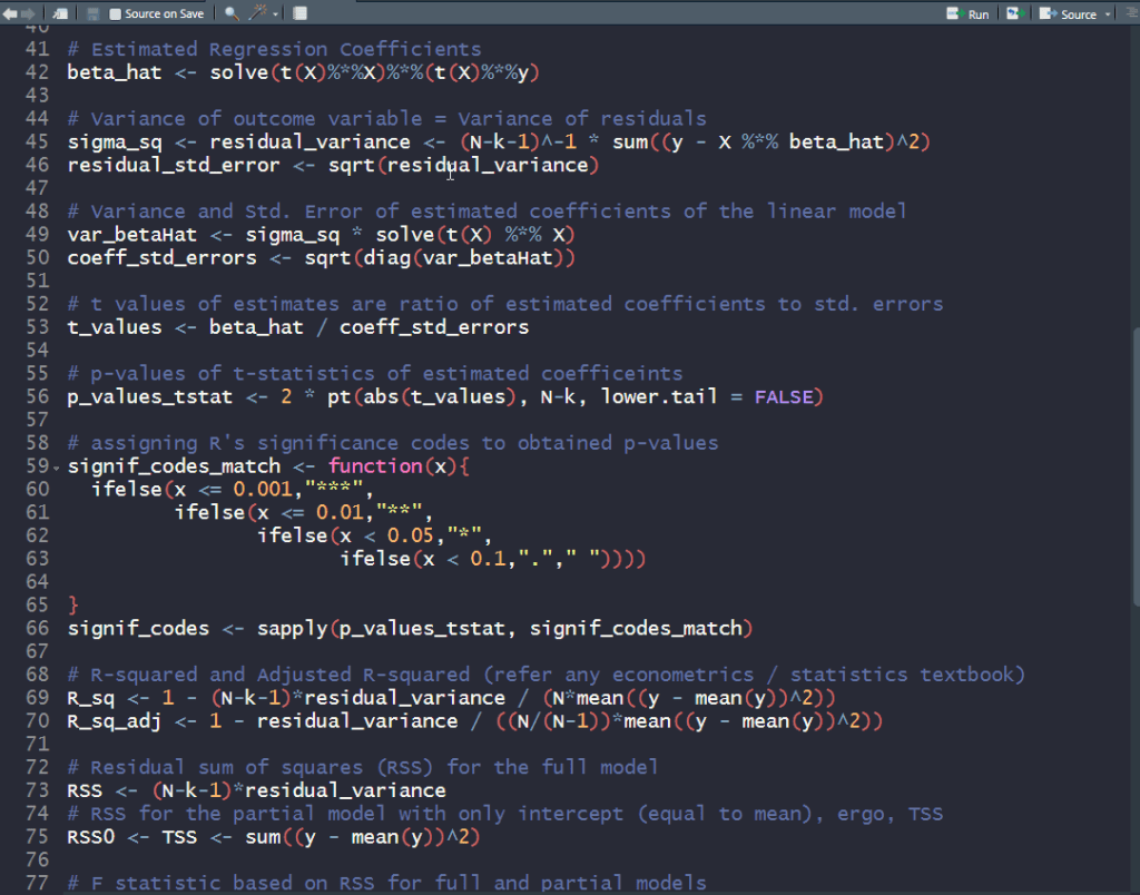
This blog post in particular was meant to be a reminder to myself and other R users that the much used lm() function in R (for fitting linear models) can be replaced with some handy matrix operations to obtain regression coefficients, their standard errors and other goodness-of-fit stats printed out when summary() is called on an lm object.

Linear regression can be formulated mathematically as follows:
\mathbf{y} = \mathbf{X} \mathbf{\beta} + \mathbf{\epsilon} ,
\mathbf{\epsilon} \sim N(0, \sigma^2 \mathbf{I})

\mathbf{y} is the \mathbf{n}\times \mathbf{1} outcome variable and \mathbf{X} is the \mathbf{n}\times \mathbf{(\mathbf{k}+1)} data matrix of independent predictor variables (including a vector of ones corresponding to the intercept). The ordinary least squares (OLS) estimate for the vector of coefficients \mathbf{\beta} is:

\hat{\mathbf{\beta}} = (\mathbf{X}^{\prime} \mathbf{X})^{-1} \mathbf{X}^{\prime} \mathbf{y}

The covariance matrix can be obtained with some handy matrix operations:
\textrm{Var}(\hat{\mathbf{\beta}}) = (\mathbf{X}^{\prime} \mathbf{X})^{-1} \mathbf{X}^{\prime} \;\sigma^2 \mathbf{I} \; \mathbf{X} (\mathbf{X}^{\prime} \mathbf{X})^{-1} = \sigma^2 (\mathbf{X}^{\prime} \mathbf{X})^{-1}
given that \textrm{Var}(AX) = A \times \textrm{Var}X \times A^{\prime}; \textrm{Var}(\mathbf{y}) = \mathbf{\sigma^2}

The standard errors of the coefficients are basically \textrm{Diag}(\sqrt{\textrm{Var}(\hat{\mathbf{\beta}})}) = \textrm{Diag}(\sqrt{\sigma^2 (\mathbf{X}^{\prime} \mathbf{X})^{-1}}) and with these, one can compute the t-statistics and their corresponding p-values.

Lastly, the F-statistic and its corresponding p-value can be calculated after computing the two residual sum of squares (RSS) statistics:

  • \mathbf{RSS} – for the full model with all predictors
  • \mathbf{RSS_0} – for the partial model (\mathbf{y} = \mathbf{\mu} + \mathbf{\nu}; \mathbf{\mu} = \mathop{\mathbb{E}}[\mathbf{y}]; \mathbf{\nu} \sim N(0, \sigma_0^2 \mathbf{I}) ) with the outcome observed mean as estimated outcome

\mathbf{F} = \frac{(\mathbf{RSS_0}-\mathbf{RSS})/\mathbf{k}}{\mathbf{RSS}/(\mathbf{n}-\mathbf{k}-1)}

I wrote some R code to construct the output from summarizing lm objects, using all the math spewed thus far. The data used for this exercise is available in R, and comprises of standardized fertility measures and socio-economic indicators for each of 47 French-speaking provinces of Switzerland from 1888. Try it out and see for yourself the linear algebra behind linear regression.

### Linear Regression Using lm() ----------------------------------------
data("swiss")
dat <- swiss
linear_model <- lm(Fertility ~ ., data = dat)
summary(linear_model)
# Call:
# lm(formula = Fertility ~ ., data = dat)
#
# Residuals:
# Min 1Q Median 3Q Max
# -15.2743 -5.2617 0.5032 4.1198 15.3213
#
# Coefficients:
# Estimate Std. Error t value Pr(>|t|)
# (Intercept) 66.91518 10.70604 6.250 1.91e-07 ***
# Agriculture -0.17211 0.07030 -2.448 0.01873 *
# Examination -0.25801 0.25388 -1.016 0.31546
# Education -0.87094 0.18303 -4.758 2.43e-05 ***
# Catholic 0.10412 0.03526 2.953 0.00519 **
# Infant.Mortality 1.07705 0.38172 2.822 0.00734 **
# ---
# Signif. codes: 0 ‘***’ 0.001 ‘**’ 0.01 ‘*’ 0.05 ‘.’ 0.1 ‘ ’ 1
#
# Residual standard error: 7.165 on 41 degrees of freedom
# Multiple R-squared: 0.7067, Adjusted R-squared: 0.671
# F-statistic: 19.76 on 5 and 41 DF, p-value: 5.594e-10
### Using Linear Algebra ------------------------------------------------
y <- matrix(dat$Fertility, nrow = nrow(dat))
X <- cbind(1, as.matrix(x = dat[,-1]))
colnames(X)[1] <- "(Intercept)"
# N x k matrix
N <- nrow(X)
k <- ncol(X) - 1 # number of predictor variables (ergo, excluding Intercept column)
# Estimated Regression Coefficients
beta_hat <- solve(t(X)%*%X)%*%(t(X)%*%y)
# Variance of outcome variable = Variance of residuals
sigma_sq <- residual_variance <- (N-k-1)^-1 * sum((y - X %*% beta_hat)^2)
residual_std_error <- sqrt(residual_variance)
# Variance and Std. Error of estimated coefficients of the linear model
var_betaHat <- sigma_sq * solve(t(X) %*% X)
coeff_std_errors <- sqrt(diag(var_betaHat))
# t values of estimates are ratio of estimated coefficients to std. errors
t_values <- beta_hat / coeff_std_errors
# p-values of t-statistics of estimated coefficeints
p_values_tstat <- 2 * pt(abs(t_values), N-k, lower.tail = FALSE)
# assigning R's significance codes to obtained p-values
signif_codes_match <- function(x){
ifelse(x <= 0.001,"***",
ifelse(x <= 0.01,"**",
ifelse(x < 0.05,"*",
ifelse(x < 0.1,"."," "))))
}
signif_codes <- sapply(p_values_tstat, signif_codes_match)
# R-squared and Adjusted R-squared (refer any econometrics / statistics textbook)
R_sq <- 1 - (N-k-1)*residual_variance / (N*mean((y - mean(y))^2))
R_sq_adj <- 1 - residual_variance / ((N/(N-1))*mean((y - mean(y))^2))
# Residual sum of squares (RSS) for the full model
RSS <- (N-k-1)*residual_variance
# RSS for the partial model with only intercept (equal to mean), ergo, TSS
RSS0 <- TSS <- sum((y - mean(y))^2)
# F statistic based on RSS for full and partial models
# k = degress of freedom of partial model
# N - k - 1 = degress of freedom of full model
F_stat <- ((RSS0 - RSS)/k) / (RSS/(N-k-1))
# p-values of the F statistic
p_value_F_stat <- pf(F_stat, df1 = k, df2 = N-k-1, lower.tail = FALSE)
# stitch the main results toghether
lm_results <- as.data.frame(cbind(beta_hat, coeff_std_errors,
t_values, p_values_tstat, signif_codes))
colnames(lm_results) <- c("Estimate","Std. Error","t value","Pr(>|t|)","")
### Print out results of all relevant calcualtions -----------------------
print(lm_results)
cat("Residual standard error: ",
round(residual_std_error, digits = 3),
" on ",N-k-1," degrees of freedom",
"\nMultiple R-squared: ",R_sq," Adjusted R-squared: ",R_sq_adj,
"\nF-statistic: ",F_stat, " on ",k-1," and ",N-k-1,
" DF, p-value: ", p_value_F_stat,"\n")
# Estimate Std. Error t value Pr(>|t|)
# (Intercept) 66.9151816789654 10.7060375853301 6.25022854119771 1.73336561301153e-07 ***
# Agriculture -0.172113970941457 0.0703039231786469 -2.44814177018405 0.0186186100433133 *
# Examination -0.258008239834722 0.253878200892098 -1.01626779663678 0.315320687313066
# Education -0.870940062939429 0.183028601571259 -4.75849159892283 2.3228265226988e-05 ***
# Catholic 0.104115330743766 0.035257852536169 2.95296858017545 0.00513556154915653 **
# Infant.Mortality 1.07704814069103 0.381719650858061 2.82156849475775 0.00726899472564356 **
# Residual standard error: 7.165 on 41 degrees of freedom
# Multiple R-squared: 0.706735 Adjusted R-squared: 0.670971
# F-statistic: 19.76106 on 4 and 41 DF, p-value: 5.593799e-10

Hope this was useful and worth your time!

Linear / Logistic Regression in R: Dealing With Unknown Factor Levels in Test Data

Let’s say you have data containing a categorical variable with 50 levels. When you divide the data into train and test sets, chances are you don’t have all 50 levels featuring in your training set.

This often happens when you divide the data set into train and test sets according to the distribution of the outcome variable. In doing so, chances are that our explanatory categorical variable might not be distributed exactly the same way in train and test sets – so much so that certain levels of this categorical variable are missing from the training set. The more levels there are to a categorical variable, it gets difficult for that variable to be similarly represented upon splitting the data.

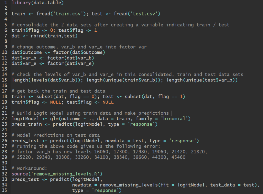
Take for instance this example data set (train.csv + test.csv) which contains a categorical variable var_b that takes 349 unique levels. Our train data has 334 of these levels – on which the model is built – and hence 15 levels are excluded from our trained model. If you try making predictions on the test set with this model in R, it throws an error:
factor var_b has new levels 16060, 17300, 17980, 19060, 21420, 21820,
25220, 29340, 30300, 33260, 34100, 38340, 39660, 44300, 45460

If you’ve used R to model generalized linear class of models such as linear, logit or probit models, then chances are you’ve come across this problem – especially when you’re validating your trained model on test data.

The workaround to this problem is in the form of a function, remove_missing_levels  that I found here written by pat-s. You need magrittr library installed and it can only work on lm, glm and glmmPQL objects.

remove_missing_levels <- function(fit, test_data) {
library(magrittr)
# https://stackoverflow.com/a/39495480/4185785
# drop empty factor levels in test data
test_data %>%
droplevels() %>%
as.data.frame() -> test_data
# 'fit' object structure of 'lm' and 'glmmPQL' is different so we need to
# account for it
if (any(class(fit) == "glmmPQL")) {
# Obtain factor predictors in the model and their levels
factors <- (gsub("[-^0-9]|as.factor|\\(|\\)", "",
names(unlist(fit$contrasts))))
# do nothing if no factors are present
if (length(factors) == 0) {
return(test_data)
}
map(fit$contrasts, function(x) names(unmatrix(x))) %>%
unlist() -> factor_levels
factor_levels %>% str_split(":", simplify = TRUE) %>%
extract(, 1) -> factor_levels
model_factors <- as.data.frame(cbind(factors, factor_levels))
} else {
# Obtain factor predictors in the model and their levels
factors <- (gsub("[-^0-9]|as.factor|\\(|\\)", "",
names(unlist(fit$xlevels))))
# do nothing if no factors are present
if (length(factors) == 0) {
return(test_data)
}
factor_levels <- unname(unlist(fit$xlevels))
model_factors <- as.data.frame(cbind(factors, factor_levels))
}
# Select column names in test data that are factor predictors in
# trained model
predictors <- names(test_data[names(test_data) %in% factors])
# For each factor predictor in your data, if the level is not in the model,
# set the value to NA
for (i in 1:length(predictors)) {
found <- test_data[, predictors[i]] %in% model_factors[
model_factors$factors == predictors[i], ]$factor_levels
if (any(!found)) {
# track which variable
var <- predictors[i]
# set to NA
test_data[!found, predictors[i]] <- NA
# drop empty factor levels in test data
test_data %>%
droplevels() -> test_data
# issue warning to console
message(sprintf(paste0("Setting missing levels in '%s', only present",
" in test data but missing in train data,",
" to 'NA'."),
var))
}
}
return(test_data)
}

Once you’ve sourced the above function in R, you can seamlessly proceed with using your trained model to make predictions on the test set. The code below demonstrates this for the data set shared above. You can find these codes in one of my github repos and try it out yourself.

library(data.table)
train <- fread('train.csv'); test <- fread('test.csv')
# consolidate the 2 data sets after creating a variable indicating train / test
train$flag <- 0; test$flag <- 1
dat <- rbind(train,test)
# change outcome, var_b and var_e into factor var
dat$outcome <- factor(dat$outcome)
dat$var_b <- factor(dat$var_b)
dat$var_e <- factor(dat$var_e)
# check the levels of var_b and var_e in this consolidated, train and test data sets
length(levels(dat$var_b)); length(unique(train$var_b)); length(unique(test$var_b))
# get back the train and test data
train <- subset(dat, flag == 0); test <- subset(dat, flag == 1)
train$flag <- NULL; test$flag <- NULL
# Build Logit Model using train data and make predictions
logitModel <- glm(outcome ~ ., data = train, family = 'binomial')
preds_train <- predict(logitModel, type = 'response')
# Model Predictions on test data
preds_test <- predict(logitModel, newdata = test, type = 'response')
# running the above code gives us the following error:
# factor var_b has new levels 16060, 17300, 17980, 19060, 21420, 21820,
# 25220, 29340, 30300, 33260, 34100, 38340, 39660, 44300, 45460
# Workaround:
source('remove_missing_levels.R')
preds_test <- predict(logitModel,
newdata = remove_missing_levels(fit = logitModel, test_data = test),
type = 'response')

Implementing Undirected Graphs in Python

There are 2 popular ways of representing an undirected graph.

Adjacency List
Each list describes the set of neighbors of a vertex in the graph.

adjacencyList

Adjacency Matrix
The elements of the matrix indicate whether pairs of vertices are adjacent or not in the graph.

adjacencyMatrix

Here’s an implementation of the above in Python:

class Vertex:
def __init__(self, vertex):
self.name = vertex
self.neighbors = []
def add_neighbor(self, neighbor):
if isinstance(neighbor, Vertex):
if neighbor.name not in self.neighbors:
self.neighbors.append(neighbor.name)
neighbor.neighbors.append(self.name)
self.neighbors = sorted(self.neighbors)
neighbor.neighbors = sorted(neighbor.neighbors)
else:
return False
def add_neighbors(self, neighbors):
for neighbor in neighbors:
if isinstance(neighbor, Vertex):
if neighbor.name not in self.neighbors:
self.neighbors.append(neighbor.name)
neighbor.neighbors.append(self.name)
self.neighbors = sorted(self.neighbors)
neighbor.neighbors = sorted(neighbor.neighbors)
else:
return False
def __repr__(self):
return str(self.neighbors)
class Graph:
def __init__(self):
self.vertices = {}
def add_vertex(self, vertex):
if isinstance(vertex, Vertex):
self.vertices[vertex.name] = vertex.neighbors
def add_vertices(self, vertices):
for vertex in vertices:
if isinstance(vertex, Vertex):
self.vertices[vertex.name] = vertex.neighbors
def add_edge(self, vertex_from, vertex_to):
if isinstance(vertex_from, Vertex) and isinstance(vertex_to, Vertex):
vertex_from.add_neighbor(vertex_to)
if isinstance(vertex_from, Vertex) and isinstance(vertex_to, Vertex):
self.vertices[vertex_from.name] = vertex_from.neighbors
self.vertices[vertex_to.name] = vertex_to.neighbors
def add_edges(self, edges):
for edge in edges:
self.add_edge(edge[0],edge[1])
def adjacencyList(self):
if len(self.vertices) >= 1:
return [str(key) + ":" + str(self.vertices[key]) for key in self.vertices.keys()]
else:
return dict()
def adjacencyMatrix(self):
if len(self.vertices) >= 1:
self.vertex_names = sorted(g.vertices.keys())
self.vertex_indices = dict(zip(self.vertex_names, range(len(self.vertex_names))))
import numpy as np
self.adjacency_matrix = np.zeros(shape=(len(self.vertices),len(self.vertices)))
for i in range(len(self.vertex_names)):
for j in range(i, len(self.vertices)):
for el in g.vertices[self.vertex_names[i]]:
j = g.vertex_indices[el]
self.adjacency_matrix[i,j] = 1
return self.adjacency_matrix
else:
return dict()
def graph(g):
""" Function to print a graph as adjacency list and adjacency matrix. """
return str(g.adjacencyList()) + '\n' + '\n' + str(g.adjacencyMatrix())
###################################################################################
a = Vertex('A')
b = Vertex('B')
c = Vertex('C')
d = Vertex('D')
e = Vertex('E')
a.add_neighbors([b,c,e])
b.add_neighbors([a,c])
c.add_neighbors([b,d,a,e])
d.add_neighbor(c)
e.add_neighbors([a,c])
g = Graph()
print(graph(g))
print()
g.add_vertices([a,b,c,d,e])
g.add_edge(b,d)
print(graph(g))

Output:

{}
{}
["A:['B', 'C', 'E']", "C:['A', 'B', 'D', 'E']", "B:['A', 'C', 'D']", "E:['A', 'C']", "D:['B', 'C']"]
[[ 0. 1. 1. 0. 1.]
[ 1. 0. 1. 1. 0.]
[ 1. 1. 0. 1. 1.]
[ 0. 1. 1. 0. 0.]
[ 1. 0. 1. 0. 0.]]

Deterministic Selection Algorithm Python Code

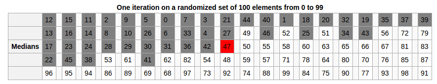
Through this post, I’m sharing Python code implementing the median of medians algorithm, an algorithm that resembles quickselect, differing only in the way in which the pivot is chosen, i.e, deterministically, instead of at random.

Its best case complexity is O(n) and worst case complexity O(nlog2n)

I don’t have a formal education in CS, and came across this algorithm while going through Tim Roughgarden’s Coursera MOOC on the design and analysis of algorithms. Check out my implementation in Python.

def merge_tuple(a,b):
""" Function to merge two arrays of tuples """
c = []
while len(a) != 0 and len(b) != 0:
if a[0][0] < b[0][0]:
c.append(a[0])
a.remove(a[0])
else:
c.append(b[0])
b.remove(b[0])
if len(a) == 0:
c += b
else:
c += a
return c
def mergesort_tuple(x):
""" Function to sort an array using merge sort algorithm """
if len(x) == 0 or len(x) == 1:
return x
else:
middle = len(x)/2
a = mergesort_tuple(x[:middle])
b = mergesort_tuple(x[middle:])
return merge_tuple(a,b)
def lol(x,k):
""" Function to divide a list into a list of lists of size k each. """
return [x[i:i+k] for i in range(0,len(x),k)]
def preprocess(x):
""" Function to assign an index to each element of a list of integers, outputting a list of tuples"""
return zip(x,range(len(x)))
def partition(x, pivot_index = 0):
""" Function to partition an unsorted array around a pivot"""
i = 0
if pivot_index !=0: x[0],x[pivot_index] = x[pivot_index],x[0]
for j in range(len(x)-1):
if x[j+1] < x[0]:
x[j+1],x[i+1] = x[i+1],x[j+1]
i += 1
x[0],x[i] = x[i],x[0]
return x,i
def ChoosePivot(x):
""" Function to choose pivot element of an unsorted array using 'Median of Medians' method. """
if len(x) <= 5:
return mergesort_tuple(x)[middle_index(x)]
else:
lst = lol(x,5)
lst = [mergesort_tuple(el) for el in lst]
C = [el[middle_index(el)] for el in lst]
return ChoosePivot(C)
def DSelect(x,k):
""" Function to """
if len(x) == 1:
return x[0]
else:
xpart = partition(x,ChoosePivot(preprocess(x))[1])
x = xpart[0] # partitioned array
j = xpart[1] # pivot index
if j == k:
return x[j]
elif j > k:
return DSelect(x[:j],k)
else:
k = k - j - 1
return DSelect(x[(j+1):], k)
arr = range(100,0,-1)
print DSelect(arr,50)
%timeit DSelect(arr,50)
view raw DSelect.py hosted with ❤ by GitHub

I get the following output:

51
100 loops, best of 3: 2.38 ms per loop

Note that on the same input, quickselect is faster, giving us:

1000 loops, best of 3: 254 µs per loop

scikit-learn Linear Regression Example

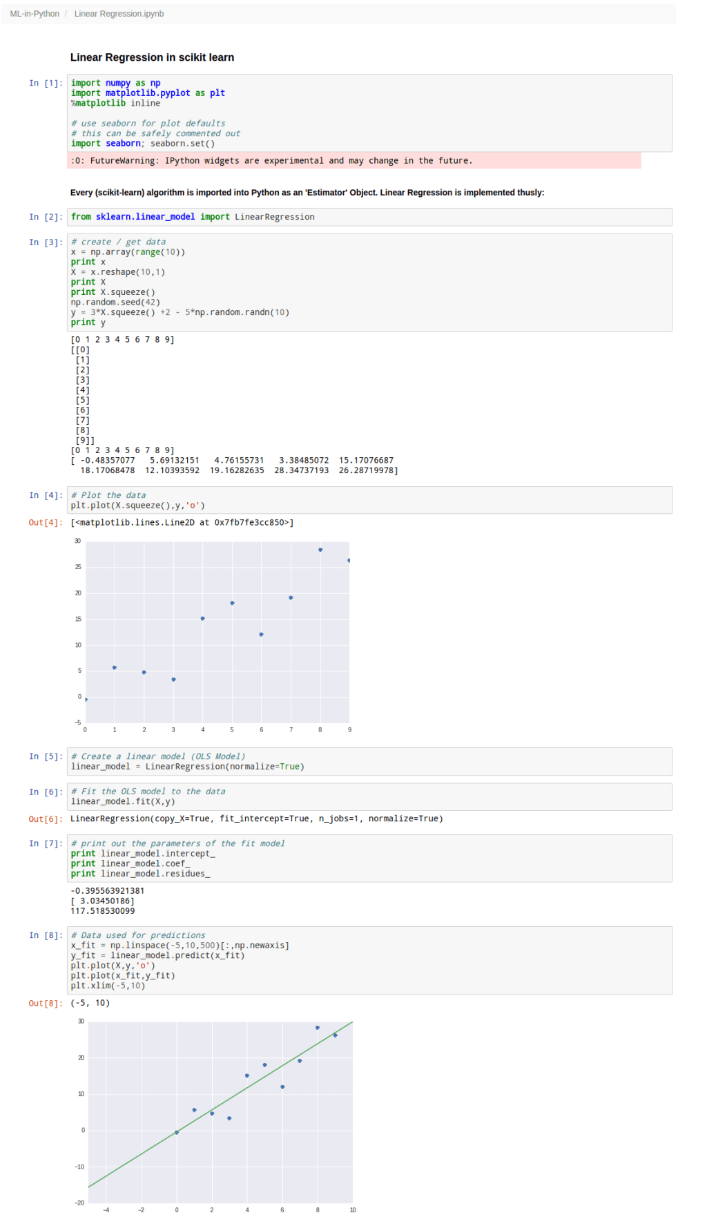
Here’s a quick example case for implementing one of the simplest of learning algorithms in any machine learning toolbox – Linear Regression. You can download the IPython / Jupyter notebook here so as to play around with the code and try things out yourself.

I’m doing a series of posts on scikit-learn. Its documentation is vast, so unless you’re willing to search for a needle in a haystack, you’re better off NOT jumping into the documentation right away. Instead, knowing chunks of code that do the job might help.

Sorry, something went wrong. Reload?
Sorry, we cannot display this file.
Sorry, this file is invalid so it cannot be displayed.

Detecting Structural Breaks in China’s FX Regime

Edit: This post is in its infancy. Work is still ongoing as far as deriving insight from the data is concerned. More content and economic insight is expected to be added to this post as and when progress is made in that direction.

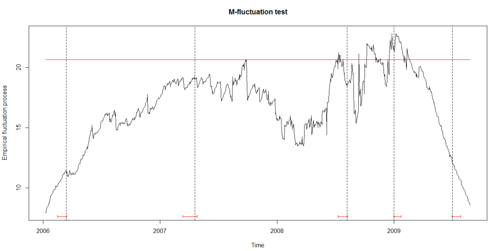
This is an attempt to detect structural breaks in China’s FX regime using Frenkel Wei regression methodology (this was later improved by Perron and Bai). I came up with the motivation to check for these structural breaks while attending a guest lecture on FX regimes by Dr. Ajay Shah delivered at IGIDR. This is work that I and two other classmates are working on as a term paper project under the supervision of Dr. Rajeswari Sengupta.

The code below can be replicated and run as is, to get same results.

## if fxregime or strucchange package is absent from installed packages, download it and load it
if(!require('fxregime')){
install.packages("fxregime")
}
if(!require('strucchange')){
install.packages("strucchange")
}
## load packages
library("fxregime")
library('strucchange')
# load the necessary data related to exchange rates - 'FXRatesCHF'
# this dataset treats CHF as unit currency
data("FXRatesCHF", package = "fxregime")
## compute returns for CNY (and explanatory currencies)
## since China abolished fixed USD regime
cny <- fxreturns("CNY", frequency = "daily",
start = as.Date("2005-07-25"), end = as.Date("2010-02-12"),
other = c("USD", "JPY", "EUR", "GBP"))
## compute all segmented regression with minimal segment size of
## h = 100 and maximal number of breaks = 10
regx <- fxregimes(CNY ~ USD + JPY + EUR + GBP,
data = cny, h = 100, breaks = 10, ic = "BIC")
## Print summary of regression results
summary(regx)
## minimum BIC is attained for 2-segment (1-break) model
plot(regx)
round(coef(regx), digits = 3)
sqrt(coef(regx)[, "(Variance)"])
## inspect associated confidence intervals
cit <- confint(regx, level = 0.9)
cit
breakdates(cit)
## plot LM statistics along with confidence interval
flm <- fxlm(CNY ~ USD + JPY + EUR + GBP, data = cny)
scus <- gefp(flm, fit = NULL)
plot(scus, functional = supLM(0.1))
## add lines related to breaks to your plot
lines(cit)

As can be seen in the figure below, the structural breaks correspond to the vertical bars. We are still working on understanding the motivations of China’s central bank in varying the degree of the managed float exchange rate.

strucchange_china_2006_2010

EDIT (May 16, 2016):

The code above uses data provided by the package itself. If you wished to replicate this analysis on data after 2010, you will have to use your own data. We used Quandl, which lets you get 10 premium datasets for free. An API key (for only 10 calls on premium datasets) is provided if you register there. Foreign exchange rate data (2000 onward till date) apparently, is premium data. You can find these here.

Here are the (partial) results and code to work the same methodology on the data from 2010 to 2016:

20102016

## if fxregime is absent from installed packages, download it and load it
if(!require('fxregime')){
install.packages("fxregime")
}
## load package
library("fxregime")
# load the necessary data related to exchange rates - 'FXRatesCHF'
# this dataset treats CHF as unit currency
# install / load Quandl
if(!require('Quandl')){
install.packages("Quandl")
}
library(Quandl)
# Extract and load currency data series with respect to CHF from Quandl
# Extract data series from Quandl. Each Quandl user will have unique api_key
# upon signing up. The freemium version allows access up to 10 fx rate data sets
# USDCHF <- Quandl("CUR/CHF", api_key="p2GsFxccPGFSw7n1-NF9")
# write.csv(USDCHF, file = "USDCHF.csv")
# USDCNY <- Quandl("CUR/CNY", api_key="p2GsFxccPGFSw7n1-NF9")
# write.csv(USDCNY, file = "USDCNY.csv")
# USDJPY <- Quandl("CUR/JPY", api_key="p2GsFxccPGFSw7n1-NF9")
# write.csv(USDJPY, file = "USDJPY.csv")
# USDEUR <- Quandl("CUR/EUR", api_key="p2GsFxccPGFSw7n1-NF9")
# write.csv(USDEUR, file = "USDEUR.csv")
# USDGBP <- Quandl("CUR/GBP", api_key="p2GsFxccPGFSw7n1-NF9")
# write.csv(USDGBP, file = "USDGBP.csv")
# load the data sets into R
USDCHF <- read.csv("G:/China's Economic Woes/USDCHF.csv")
USDCHF <- USDCHF[,2:3]
USDCNY <- read.csv("G:/China's Economic Woes/USDCNY.csv")
USDCNY <- USDCNY[,2:3]
USDEUR <- read.csv("G:/China's Economic Woes/USDEUR.csv")
USDEUR <- USDEUR[,2:3]
USDGBP <- read.csv("G:/China's Economic Woes/USDGBP.csv")
USDGBP <- USDGBP[,2:3]
USDJPY <- read.csv("G:/China's Economic Woes/USDJPY.csv")
USDJPY <- USDJPY[,2:3]
start = 1 # corresponds to 2016-05-12
end = 2272 # corresponds to 2010-02-12
dates <- as.Date(USDCHF[start:end,1])
USD <- 1/USDCHF[start:end,2]
CNY <- USDCNY[start:end,2]/USD
JPY <- USDJPY[start:end,2]/USD
EUR <- USDEUR[start:end,2]/USD
GBP <- USDGBP[start:end,2]/USD
# reverse the order of the vectors to reflect dates from 2005 - 2010 instead of
# the other way around
USD <- USD[length(USD):1]
CNY <- CNY[length(CNY):1]
JPY <- JPY[length(JPY):1]
EUR <- EUR[length(EUR):1]
GBP <- GBP[length(GBP):1]
dates <- dates[length(dates):1]
df <- data.frame(CNY, USD, JPY, EUR, GBP)
df$weekday <- weekdays(dates)
row.names(df) <- dates
df <- subset(df, weekday != 'Sunday')
df <- subset(df, weekday != 'Saturday')
df <- df[,1:5]
zoo_df <- as.zoo(df)
# Code to replicate analysis
cny_rep <- fxreturns("CNY", data = zoo_df, frequency = "daily",
other = c("USD", "JPY", "EUR", "GBP"))
time(cny_rep) <- as.Date(row.names(df)[2:1627])
regx_rep <- fxregimes(CNY ~ USD + JPY + EUR + GBP,
data = cny_rep, h = 100, breaks = 10, ic = "BIC")
summary(regx_rep)
## minimum BIC is attained for 2-segment (5-break) model
plot(regx_rep)
round(coef(regx_rep), digits = 3)
sqrt(coef(regx_rep)[, "(Variance)"])
## inspect associated confidence intervals
cit_rep <- confint(regx_rep, level = 0.9)
breakdates(cit_rep)
## plot LM statistics along with confidence interval
flm_rep <- fxlm(CNY ~ USD + JPY + EUR + GBP, data = cny_rep)
scus_rep <- gefp(flm_rep, fit = NULL)
plot(scus_rep, functional = supLM(0.1))
## add lines related to breaks to your plot
lines(cit_rep)
apply(cny_rep,1,function(x) sum(is.na(x)))

We got breaks in 2010 and in 2015 (when China’s stock markets crashed). We would have hoped for more breaks (we can still get them), but that would depend on the parameters chosen for our regression.


Data Manipulation in R with dplyr – Part 3

This happens to be my 50th blog post – and my blog is 8 months old.

🙂

This post is the third and last post in in a series of posts (Part 1Part 2) on data manipulation with dlpyr. Note that the objects in the code may have been defined in earlier posts and the code in this post is in continuation with code from the earlier posts.

Although datasets can be manipulated in sophisticated ways by linking the 5 verbs of dplyr in conjunction, linking verbs together can be a bit verbose.

Creating multiple objects, especially when working on a large dataset can slow you down in your analysis. Chaining functions directly together into one line of code is difficult to read. This is sometimes called the Dagwood sandwich problem: you have too much filling (too many long arguments) between your slices of bread (parentheses). Functions and arguments get further and further apart.

The %>% operator allows you to extract the first argument of a function from the arguments list and put it in front of it, thus solving the Dagwood sandwich problem.

# %>% OPERATOR ----------------------------------------------------------------------
# with %>% operator
hflights %>%
mutate(diff = TaxiOut - TaxiIn) %>%
filter(!is.na(diff)) %>%
summarise(avg = mean(diff))
# without %>% operator
# arguments get further and further apart
summarize(filter(mutate(hflights, diff = TaxiOut - TaxiIn),!is.na(diff)),
avg = mean(diff))
# with %>% operator
d <- hflights %>%
select(Dest, UniqueCarrier, Distance, ActualElapsedTime) %>%
mutate(RealTime = ActualElapsedTime + 100, mph = Distance/RealTime*60)
# without %>% operator
d <- mutate(select(hflights, Dest, UniqueCarrier, Distance, ActualElapsedTime),
RealTime = ActualElapsedTime + 100, mph = Distance/RealTime*60)
# Filter and summarise d
d %>%
filter(!is.na(mph), mph < 70) %>%
summarise(n_less = n(), n_dest = n_distinct(Dest),
min_dist = min(Distance), max_dist = max(Distance))
# Let's define preferable flights as flights that are 150% faster than driving,
# i.e. that travel 105 mph or greater in real time. Also, assume that cancelled or
# diverted flights are less preferable than driving.
# ADVANCED PIPING EXERCISES
# Use one single piped call to print a summary with the following variables:
# n_non - the number of non-preferable flights in hflights,
# p_non - the percentage of non-preferable flights in hflights,
# n_dest - the number of destinations that non-preferable flights traveled to,
# min_dist - the minimum distance that non-preferable flights traveled,
# max_dist - the maximum distance that non-preferable flights traveled
hflights %>%
mutate(RealTime = ActualElapsedTime + 100, mph = Distance/RealTime*60) %>%
filter(mph < 105 | Cancelled == 1 | Diverted == 1) %>%
summarise(n_non = n(), p_non = 100*n_non/nrow(hflights), n_dest = n_distinct(Dest),
min_dist = min(Distance), max_dist = max(Distance))
# Use summarise() to create a summary of hflights with a single variable, n,
# that counts the number of overnight flights. These flights have an arrival
# time that is earlier than their departure time. Only include flights that have
# no NA values for both DepTime and ArrTime in your count.
hflights %>%
mutate(overnight = (ArrTime < DepTime)) %>%
filter(overnight == TRUE) %>%
summarise(n = n())

group_by()

group_by() defines groups within a data set. Its influence becomes clear when calling summarise() on a grouped dataset. Summarizing statistics are calculated for the different groups separately.

# group_by() -------------------------------------------------------------------------
# Generate a per-carrier summary of hflights with the following variables: n_flights,
# the number of flights flown by the carrier; n_canc, the number of cancelled flights;
# p_canc, the percentage of cancelled flights; avg_delay, the average arrival delay of
# flights whose delay does not equal NA. Next, order the carriers in the summary from
# low to high by their average arrival delay. Use percentage of flights cancelled to
# break any ties. Which airline scores best based on these statistics?
hflights %>%
group_by(UniqueCarrier) %>%
summarise(n_flights = n(), n_canc = sum(Cancelled), p_canc = 100*n_canc/n_flights,
avg_delay = mean(ArrDelay, na.rm = TRUE)) %>% arrange(avg_delay)
# Generate a per-day-of-week summary of hflights with the variable avg_taxi,
# the average total taxiing time. Pipe this summary into an arrange() call such
# that the day with the highest avg_taxi comes first.
hflights %>%
group_by(DayOfWeek) %>%
summarize(avg_taxi = mean(TaxiIn + TaxiOut, na.rm = TRUE)) %>%
arrange(desc(avg_taxi))
view raw group_by.R hosted with ❤ by GitHub

Combine group_by with mutate

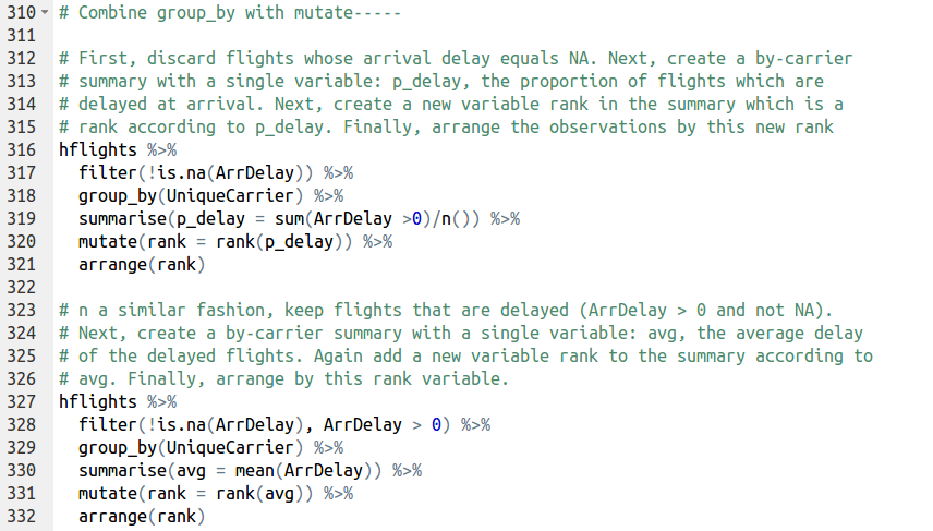
group_by() can also be combined with mutate(). When you mutate grouped data, mutate() will calculate the new variables independently for each group. This is particularly useful when mutate() uses the rank() function, that calculates within group rankings. rank() takes a group of values and calculates the rank of each value within the group, e.g.

rank(c(21, 22, 24, 23))

has output

[1] 1 2 4 3

As with arrange(), rank() ranks values from the largest to the smallest and this behaviour can be reversed with the desc() function.

# Combine group_by with mutate-----
# First, discard flights whose arrival delay equals NA. Next, create a by-carrier
# summary with a single variable: p_delay, the proportion of flights which are
# delayed at arrival. Next, create a new variable rank in the summary which is a
# rank according to p_delay. Finally, arrange the observations by this new rank
hflights %>%
filter(!is.na(ArrDelay)) %>%
group_by(UniqueCarrier) %>%
summarise(p_delay = sum(ArrDelay >0)/n()) %>%
mutate(rank = rank(p_delay)) %>%
arrange(rank)
# n a similar fashion, keep flights that are delayed (ArrDelay > 0 and not NA).
# Next, create a by-carrier summary with a single variable: avg, the average delay
# of the delayed flights. Again add a new variable rank to the summary according to
# avg. Finally, arrange by this rank variable.
hflights %>%
filter(!is.na(ArrDelay), ArrDelay > 0) %>%
group_by(UniqueCarrier) %>%
summarise(avg = mean(ArrDelay)) %>%
mutate(rank = rank(avg)) %>%
arrange(rank)
# Advanced group_by exercises-------------------------------------------------------
# Which plane (by tail number) flew out of Houston the most times? How many times?
# Name the column with this frequency n. Assign the result to adv1. To answer this
# question precisely, you will have to filter() as a final step to end up with only
# a single observation in adv1.
# Which plane (by tail number) flew out of Houston the most times? How many times? adv1
adv1 <- hflights %>%
group_by(TailNum) %>%
summarise(n = n()) %>%
filter(n == max(n))
# How many airplanes only flew to one destination from Houston? adv2
# How many airplanes only flew to one destination from Houston?
# Save the resulting dataset in adv2, that contains only a single column,
# named nplanes and a single row.
adv2 <- hflights %>%
group_by(TailNum) %>%
summarise(n_dest = n_distinct(Dest)) %>%
filter(n_dest == 1) %>%
summarise(nplanes = n())
# Find the most visited destination for each carrier and save your solution to adv3.
# Your solution should contain four columns:
# UniqueCarrier and Dest,
# n, how often a carrier visited a particular destination,
# rank, how each destination ranks per carrier. rank should be 1 for every row,
# as you want to find the most visited destination for each carrier.
adv3 <- hflights %>%
group_by(UniqueCarrier, Dest) %>%
summarise(n = n()) %>%
mutate(rank = rank(desc(n))) %>%
filter(rank == 1)
# Find the carrier that travels to each destination the most: adv4
# For each destination, find the carrier that travels to that destination the most.
# Store the result in adv4. Again, your solution should contain 4 columns:
# Dest, UniqueCarrier, n and rank.
adv4 <- hflights %>%
group_by(Dest, UniqueCarrier) %>%
summarise(n = n()) %>%
mutate(rank = rank(desc(n))) %>%
filter(rank == 1)


Data Manipulation in R with dplyr – Part 2

Note that this post is in continuation with Part 1 of this series of posts on data manipulation with dplyr in R. The code in this post carries forward from the variables / objects defined in Part 1.

In the previous post, I talked about how dplyr provides a grammar of sorts to manipulate data, and consists of 5 verbs to do so:

The 5 verbs of dplyr
select – removes columns from a dataset
filter – removes rows from a dataset
arrange – reorders rows in a dataset
mutate – uses the data to build new columns and values
summarize – calculates summary statistics

I went on to discuss examples using select() and mutate(). Let’s now talk about filter(). R comes with a set of logical operators that you can use inside filter(). These operators are:
x < y, TRUE if x is less than y
x <= y, TRUE if x is less than or equal to y
x == y, TRUE if x equals y
x != y, TRUE if x does not equal y
x >= y, TRUE if x is greater than or equal to y
x > y, TRUE if x is greater than y
x %in% c(a, b, c), TRUE if x is in the vector c(a, b, c)

The following call, for example, filters df such that only the observations where the variable a is greater than the variable b:
filter(df, a > b)

# Print out all flights in hflights that traveled 3000 or more miles
filter(hflights, Distance > 3000)
# All flights flown by one of JetBlue, Southwest, or Delta
filter(hflights, UniqueCarrier %in% c('JetBlue', 'Southwest', 'Delta'))
# All flights where taxiing took longer than flying
filter(hflights, TaxiIn + TaxiOut > AirTime)
view raw verbs05.r hosted with ❤ by GitHub

Combining tests using boolean operators
R also comes with a set of boolean operators that you can use to combine multiple logical tests into a single test. These include & (and), | (or), and ! (not). Instead of using the & operator, you can also pass several logical tests to filter(), separated by commas. The following calls equivalent:

filter(df, a > b & c > d)
filter(df, a > b, c > d)

The is.na() will also come in handy very often. This expression, for example, keeps the observations in df for which the variable x is not NA:

filter(df, !is.na(x))

# Combining tests using boolean operators
# All flights that departed before 5am or arrived after 10pm
filter(hflights, DepTime < 500 | ArrTime > 2200 )
# All flights that departed late but arrived ahead of schedule
filter(hflights, DepDelay > 0 & ArrDelay < 0)
# All cancelled weekend flights
filter(hflights, DayOfWeek %in% c(6,7) & Cancelled == 1)
# All flights that were cancelled after being delayed
filter(hflights, Cancelled == 1, DepDelay > 0)
view raw verbs06.r hosted with ❤ by GitHub

A recap on select(), mutate() and filter():

# Summarizing Exercise
# Select the flights that had JFK as their destination: c1
c1 <- filter(hflights, Dest == 'JFK')
# Combine the Year, Month and DayofMonth variables to create a Date column: c2
c2 <- mutate(c1, Date = paste(Year, Month, DayofMonth, sep = "-"))
# Print out a selection of columns of c2
select(c2, Date, DepTime, ArrTime, TailNum)
# How many weekend flights flew a distance of more than 1000 miles
# but had a total taxiing time below 15 minutes?
nrow(filter(hflights, DayOfWeek %in% c(6,7), Distance > 1000, TaxiIn + TaxiOut < 15))
view raw verbs07.r hosted with ❤ by GitHub

Arranging Data
arrange() can be used to rearrange rows according to any type of data. If you pass arrange() a character variable, R will rearrange the rows in alphabetical order according to values of the variable. If you pass a factor variable, R will rearrange the rows according to the order of the levels in your factor (running levels() on the variable reveals this order).

By default, arrange() arranges the rows from smallest to largest. Rows with the smallest value of the variable will appear at the top of the data set. You can reverse this behaviour with the desc() function. arrange() will reorder the rows from largest to smallest values of a variable if you wrap the variable name in desc() before passing it to arrange()

# Definition of dtc
dtc <- filter(hflights, Cancelled == 1, !is.na(DepDelay))
# Arrange dtc by departure delays
arrange(dtc, DepDelay)
# Arrange dtc so that cancellation reasons are grouped
arrange(dtc, CancellationCode)
# Arrange dtc according to carrier and departure delays
arrange(dtc, UniqueCarrier, DepDelay)
# Arrange according to carrier and decreasing departure delays
arrange(hflights, UniqueCarrier, desc(DepDelay))
# Arrange flights by total delay (normal order).
arrange(hflights, DepDelay + ArrDelay)
# Keep flights leaving to DFW before 8am and arrange according to decreasing AirTime
arrange(filter(hflights, Dest == 'DFW', DepTime < 800), desc(AirTime))
view raw verbs08.r hosted with ❤ by GitHub

Summarizing Data

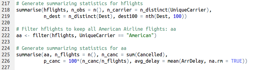
summarise(), the last of the 5 verbs, follows the same syntax as mutate(), but the resulting dataset consists of a single row instead of an entire new column in the case of mutate().

In contrast to the four other data manipulation functions, summarise() does not return an altered copy of the dataset it is summarizing; instead, it builds a new dataset that contains only the summarizing statistics.

Note: summarise() and summarize() both work the same!

You can use any function you like in summarise(), so long as the function can take a vector of data and return a single number. R contains many aggregating functions. Here are some of the most useful:

min(x) – minimum value of vector x.
   max(x) – maximum value of vector x.
mean(x) – mean value of vector x.
median(x) – median value of vector x.
quantile(x, p) – pth quantile of vector x.
  sd(x) – standard deviation of vector x.
var(x) – variance of vector x.
IQR(x) – Inter Quartile Range (IQR) of vector x.
diff(range(x)) – total range of vector x.

# Print out a summary with variables min_dist and max_dist
summarize(hflights, min_dist = min(Distance), max_dist = max(Distance))
# Print out a summary with variable max_div
summarize(filter(hflights, Diverted == 1), max_div = max(Distance))
# Remove rows that have NA ArrDelay: temp1
temp1 <- filter(hflights, !is.na(ArrDelay))
# Generate summary about ArrDelay column of temp1
summarise(temp1, earliest = min(ArrDelay), average = mean(ArrDelay),
latest = max(ArrDelay), sd = sd(ArrDelay))
# Keep rows that have no NA TaxiIn and no NA TaxiOut: temp2
temp2 <- filter(hflights, !is.na(TaxiIn), !is.na(TaxiOut))
# Print the maximum taxiing difference of temp2 with summarise()
summarise(temp2, max_taxi_diff = max(abs(TaxiIn - TaxiOut)))
view raw verbs09.r hosted with ❤ by GitHub

dplyr provides several helpful aggregate functions of its own, in addition to the ones that are already defined in R. These include:

first(x) – The first element of vector x.
last(x) – The last element of vector x.
nth(x, n) – The nth element of vector x.
n() – The number of rows in the data.frame or group of observations that summarise() describes.
n_distinct(x) – The number of unique values in vector x

# Generate summarizing statistics for hflights
summarise(hflights, n_obs = n(), n_carrier = n_distinct(UniqueCarrier),
n_dest = n_distinct(Dest), dest100 = nth(Dest, 100))
# Filter hflights to keep all American Airline flights: aa
aa <- filter(hflights, UniqueCarrier == "American")
# Generate summarizing statistics for aa
summarise(aa, n_flights = n(), n_canc = sum(Cancelled),
p_canc = 100*(n_canc/n_flights), avg_delay = mean(ArrDelay, na.rm = TRUE))
view raw verbs10.r hosted with ❤ by GitHub

This would be it for Part-2 of this series of posts on data manipulation with dplyr. Part 3 would focus on the pipe operator, Group_by and working with databases.

Data Manipulation in R with dplyr – Part 1

dplyr is one of the packages in R that makes R so loved by data scientists. It has three main goals:

  1. Identify the most important data manipulation tools needed for data analysis and make them easy to use in R.
  2. Provide blazing fast performance for in-memory data by writing key pieces of code in C++.
  3. Use the same code interface to work with data no matter where it’s stored, whether in a data frame, a data table or database.

Introduction to the dplyr package and the tbl class
This post is mostly about code. If you’re interested in learning dplyr I recommend you type in the commands line by line on the R console to see first hand what’s happening.

# INTRODUCTION TO dplyr AND tbls
# Load the dplyr package
library(dplyr)
# Load the hflights package
library(hflights)
# Call both head() and summary() on hflights
head(hflights)
summary(hflights)
# Convert the hflights data.frame into a hflights tbl
hflights <- tbl_df(hflights)
# Display the hflights tbl
hflights
# Create the object carriers, containing only the UniqueCarrier variable of hflights
carriers <- hflights$UniqueCarrier
# Use lut to translate the UniqueCarrier column of hflights and before doing so
# glimpse hflights to see the UniqueCarrier variablle
glimpse(hflights)
lut <- c("AA" = "American", "AS" = "Alaska", "B6" = "JetBlue", "CO" = "Continental",
"DL" = "Delta", "OO" = "SkyWest", "UA" = "United", "US" = "US_Airways",
"WN" = "Southwest", "EV" = "Atlantic_Southeast", "F9" = "Frontier",
"FL" = "AirTran", "MQ" = "American_Eagle", "XE" = "ExpressJet", "YV" = "Mesa")
hflights$UniqueCarrier <- lut[hflights$UniqueCarrier]
# Now glimpse hflights to see the change in the UniqueCarrier variable
glimpse(hflights)
# Fill up empty entries of CancellationCode with 'E'
# To do so, first index the empty entries in CancellationCode
cancellationEmpty <- hflights$CancellationCode == ""
# Assign 'E' to the empty entries
hflights$CancellationCode[cancellationEmpty] <- 'E'
# Use a new lookup table to create a vector of code labels. Assign the vector to the CancellationCode column of hflights
lut = c('A' = 'carrier', 'B' = 'weather', 'C' = 'FFA', 'D' = 'security', 'E' = 'not cancelled')
hflights$CancellationCode <- lut[hflights$CancellationCode]
# Inspect the resulting raw values of your variables
glimpse(hflights)
view raw introduction.R hosted with ❤ by GitHub

Select and mutate
dplyr provides grammar for data manipulation apart from providing data structure. The grammar is built around 5 functions (also referred to as verbs) that do the basic tasks of data manipulation.

The 5 verbs of dplyr
select – removes columns from a dataset
filter – removes rows from a dataset
arrange – reorders rows in a dataset
mutate – uses the data to build new columns and values
summarize – calculates summary statistics

dplyr functions do not change the dataset. They return a new copy of the dataset to use.

To answer the simple question whether flight delays tend to shrink or grow during a flight, we can safely discard a lot of the variables of each flight. To select only the ones that matter, we can use select()

hflights[c('ActualElapsedTime','ArrDelay','DepDelay')]
# Equivalently, using dplyr:
select(hflights, ActualElapsedTime, ArrDelay, DepDelay)
# Print out a tbl with the four columns of hflights related to delay
select(hflights, ActualElapsedTime, AirTime, ArrDelay, DepDelay)
# Print out hflights, nothing has changed!
hflights
# Print out the columns Origin up to Cancelled of hflights
select(hflights, Origin:Cancelled)
# Find the most concise way to select: columns Year up to and
# including DayOfWeek, columns ArrDelay up to and including Diverted
# Answer to last question: be concise!
# You may want to examine the order of hflight's column names before you
# begin with names()
names(hflights)
select(hflights, -(DepTime:AirTime))
view raw verbs01.R hosted with ❤ by GitHub

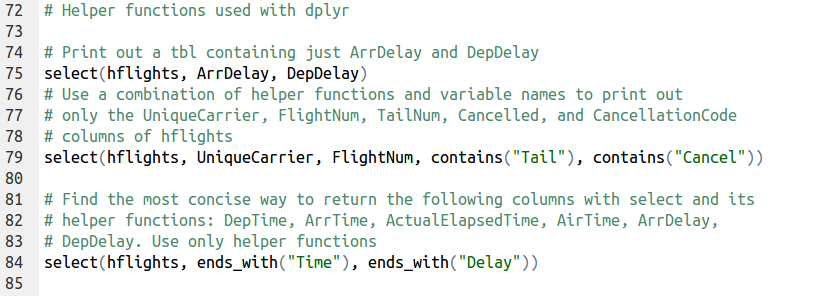
dplyr comes with a set of helper functions that can help you select variables. These functions find groups of variables to select, based on their names. Each of these works only when used inside of select()

  • starts_with(“X”): every name that starts with “X”
  • ends_with(“X”): every name that ends with “X”
  • contains(“X”): every name that contains “X”
  • matches(“X”): every name that matches “X”, where “X” can be a regular expression
  • num_range(“x”, 1:5): the variables named x01, x02, x03, x04 and x05
  • one_of(x): every name that appears in x, which should be a character vector
# Helper functions used with dplyr
# Print out a tbl containing just ArrDelay and DepDelay
select(hflights, ArrDelay, DepDelay)
# Use a combination of helper functions and variable names to print out
# only the UniqueCarrier, FlightNum, TailNum, Cancelled, and CancellationCode
# columns of hflights
select(hflights, UniqueCarrier, FlightNum, contains("Tail"), contains("Cancel"))
# Find the most concise way to return the following columns with select and its
# helper functions: DepTime, ArrTime, ActualElapsedTime, AirTime, ArrDelay,
# DepDelay. Use only helper functions
select(hflights, ends_with("Time"), ends_with("Delay"))
view raw verbs02.R hosted with ❤ by GitHub

In order to appreciate the usefulness of dplyr, here are some comparisons between base R and dplyr

# Some comparisons to basic R
# both hflights and dplyr are available
ex1r <- hflights[c("TaxiIn","TaxiOut","Distance")]
ex1d <- select(hflights, TaxiIn, TaxiOut, Distance)
ex2r <- hflights[c("Year","Month","DayOfWeek","DepTime","ArrTime")]
ex2d <- select(hflights, Year:ArrTime, -DayofMonth)
ex3r <- hflights[c("TailNum","TaxiIn","TaxiOut")]
ex3d <- select(hflights, TailNum, contains("Taxi"))
view raw comparisons01.R hosted with ❤ by GitHub

mutate() is the second of the five data manipulation functions. mutate() creates new columns which are added to a copy of the dataset.

# Add the new variable ActualGroundTime to a copy of hflights and save the result as g1.
g1 <- mutate(hflights, ActualGroundTime = ActualElapsedTime - AirTime)
# Add the new variable GroundTime to a g1. Save the result as g2.
g2 <- mutate(g1, GroundTime = TaxiIn + TaxiOut)
# Add the new variable AverageSpeed to g2. Save the result as g3.
g3 <- mutate(g2, AverageSpeed = Distance / AirTime * 60)
# Print out g3
g3
view raw verbs03.r hosted with ❤ by GitHub

So far we have added variables to hflights one at a time, but we can also use mutate() to add multiple variables at once.

# Add a second variable loss_percent to the dataset: m1
m1 <- mutate(hflights, loss = ArrDelay - DepDelay, loss_percent = ((ArrDelay - DepDelay)/DepDelay)*100)
# mutate() allows you to use a new variable while creating a next variable in the same call
# Copy and adapt the previous command to reduce redendancy: m2
m2 <- mutate(hflights, loss = ArrDelay - DepDelay, loss_percent = (loss/DepDelay) * 100 )
# Add the three variables as described in the third instruction: m3
m3 <- mutate(hflights, TotalTaxi = TaxiIn + TaxiOut, ActualGroundTime = ActualElapsedTime - AirTime, Diff = TotalTaxi - ActualGroundTime)
view raw verbs04.r hosted with ❤ by GitHub