I recently got myself to start using Python on Windows, whereas till very recently I had been working on Python only from Ubuntu.
I am sure I am late in realizing this, but installing Tensorflow was just so easy!
If you’ve tried installing Tensorflow for Windows when it was first introduced, and gave up back then – try again. The method I’d recommend would be using Anaconda Navigator from where you first open a terminal (figure below). You may notice that I already have a tensorflow environment set up, since I am writing this post after installation.
Once you have terminal open, create a conda environment named tensorflow by invoking the following command, with your python version:
C:> conda create -n tensorflow python=3.6
That’s all! You should now have tensorflow ready to use.
For more details, you could always go here. Otherwise, the screenshot below gives a sense of what it takes.
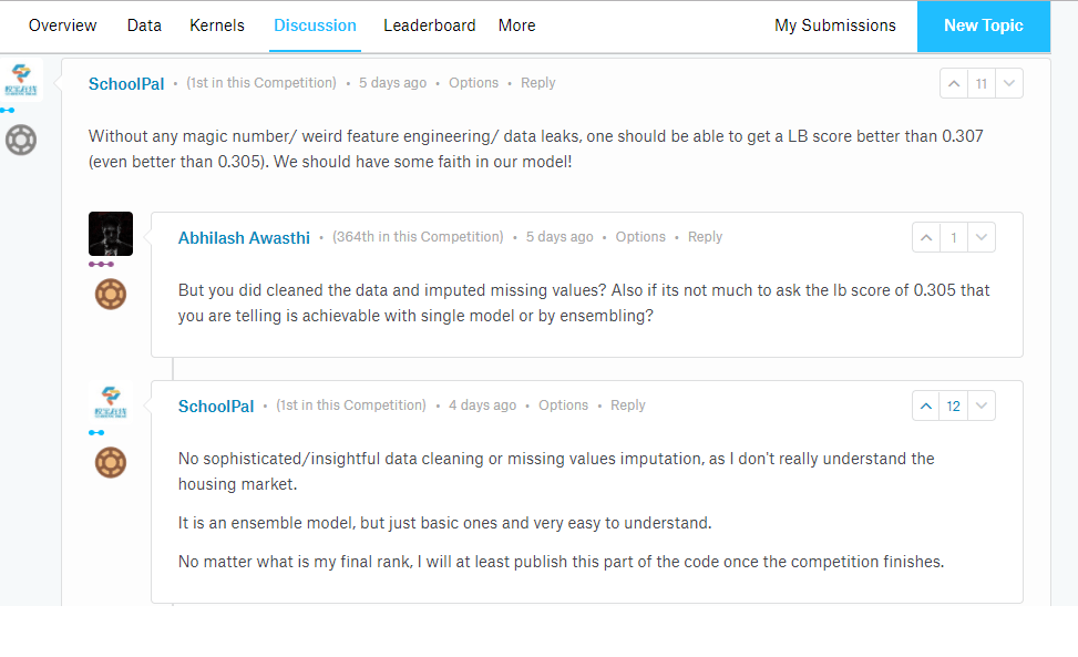
I’ve been stuck for about a week at the 52nd percentile among 3400+ Kagglers taking part in the competition. I’ve been told that Kaggle Kernels and discussion boards are helpful when you’re stuck or if you need to learn some practical data science that can’t be gleaned from books or tutorials.
One such discussion thread looks like this:
This person going by the pseudonym Schoolpal is currently killing it on the leaderboard and I’m eagerly looking forward to this person’s code once the competition ends in less than 24 hours. If you’re interested too, follow this discussion here.
Cheers!
Update:
This Schoolpal, as mentioned earlier, finally came in second and shared their approach here.
I love probability and have solved countless problems on probability ever since I learned math
…and yet I’ve never coded up probabilistic models!
The assignments and project work for this course are to be implemented in Python!
You don’t need to have prior experience in either probability or inference, but you should be comfortable with basic Python programming and calculus.
WHAT YOU’LL LEARN
– Basic discrete probability theory
– Graphical models as a data structure for representing probability distributions
– Algorithms for prediction and inference
– How to model real-world problems in terms of probabilistic inference
The course started on September 12, is 12-weeks long and is structured in the following manner:
Week 1 (9/12 – 9/16): Introduction to probability and computation
A first look at basic discrete probability, how to interpret it, what probability spaces and random variables are, and how to code these up and do basic simulations and visualizations.
Week 2 (9/19 – 9/23):Incorporating observations
Incorporating observations using jointly distributed random variables and using events. Three classic probability puzzles are presented to help elucidate how to interpret probability: Simpson’s paradox, Monty Hall, boy or girl paradox.
Week 3 (9/26 – 9/30):Introduction to inference, structure in distributions, and information measures
The product rule and inference with Bayes’ theorem. Independence: A structure in distributions. Measures of randomness: entropy and information divergence. Mutual information.
Week 4 (10/3 – 10/7):Expectations, and driving to infinity in modeling uncertainty
Expected values of random variables. Classic puzzle: the two envelope problem. Probability spaces and random variables that take on a countably infinite number of values and inference with these random variables.
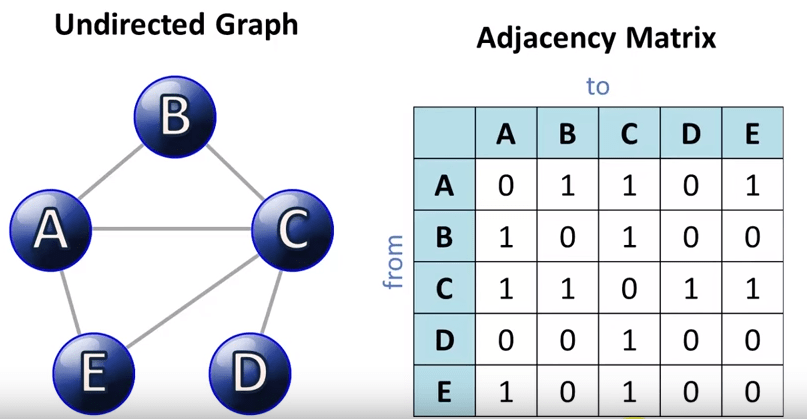
Week 5 (10/10 – 10/14):Efficient representations of probability distributions on a computer
Introduction to undirected graphical models as a data structure for representing probability distributions and the benefits/drawbacks of these graphical models. Incorporating observations with graphical models.
Week 6 (10/17 – 10/21):Inference with graphical models, part I
Computing marginal distributions with graphical models in undirected graphical models including hidden Markov models..
Week 7 (10/24 – 10/28):Inference with graphical models, part II
Computing most probable configurations with graphical models including hidden Markov models.
Week 8 (10/31 – 11/4):Introduction to learning probability distributions
Learning an underlying unknown probability distribution from observations using maximum likelihood. Three examples: estimating the bias of a coin, the German tank problem, and email spam detection.
Week 9 (11/7 – 11/11):Parameter estimation in graphical models
Given the graph structure of an undirected graphical model, we examine how to estimate all the tables associated with the graphical model.
Week 10 (11/14 – 11/18):Model selection with information theory
Learning both the graph structure and the tables of an undirected graphical model with the help of information theory. Mutual information of random variables.
Week 11 (11/21 – 11/25):Final project
Final project assigned
Week 12 (11/28 – 12/2):Final project
I’m SO taking this course. Hope this interests you as well!
This was a hackathon + workshop conducted by Analytics Vidhya in which I took part and made it to the #1 on the leaderboard. The data set was straight-forward and quite clean with only a minor need for missing value treatment. This post will might be useful for people who want a walk-through on the steps involving data munging and developing machine-learned models.
The workshop ended with a basic hackathon with data given on age, education, working class, occupation, marital status and gender of individuals and one had to predict the income bracket of these individuals.
I’ve posted the data and my code and solutions in this GitHub repo. An IPython Notebook has also been shared.
I approached the problem first by attempting some feature engineering (other than missing value treatment) on the data, and then ran a basic logistic classifier and a random forest classifier. However it turned out that these models performed better without feature engineering, which shows the dataset was already quite clean and informative to begin with for this competition.
I later attempted gradient boosting with parameter tuning to maximizing scores.
This file contains hidden or bidirectional Unicode text that may be interpreted or compiled differently than what appears below. To review, open the file in an editor that reveals hidden Unicode characters.
Learn more about bidirectional Unicode characters
This file contains hidden or bidirectional Unicode text that may be interpreted or compiled differently than what appears below. To review, open the file in an editor that reveals hidden Unicode characters.
Learn more about bidirectional Unicode characters
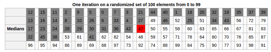
Through this post, I’m sharing Python code implementing the median of medians algorithm, an algorithm that resembles quickselect, differing only in the way in which the pivot is chosen, i.e, deterministically, instead of at random.
Its best case complexity is O(n) and worst case complexity O(nlog2n)
I don’t have a formal education in CS, and came across this algorithm while going through Tim Roughgarden’s Coursera MOOC on the design and analysis of algorithms. Check out my implementation in Python.
This file contains hidden or bidirectional Unicode text that may be interpreted or compiled differently than what appears below. To review, open the file in an editor that reveals hidden Unicode characters.
Learn more about bidirectional Unicode characters
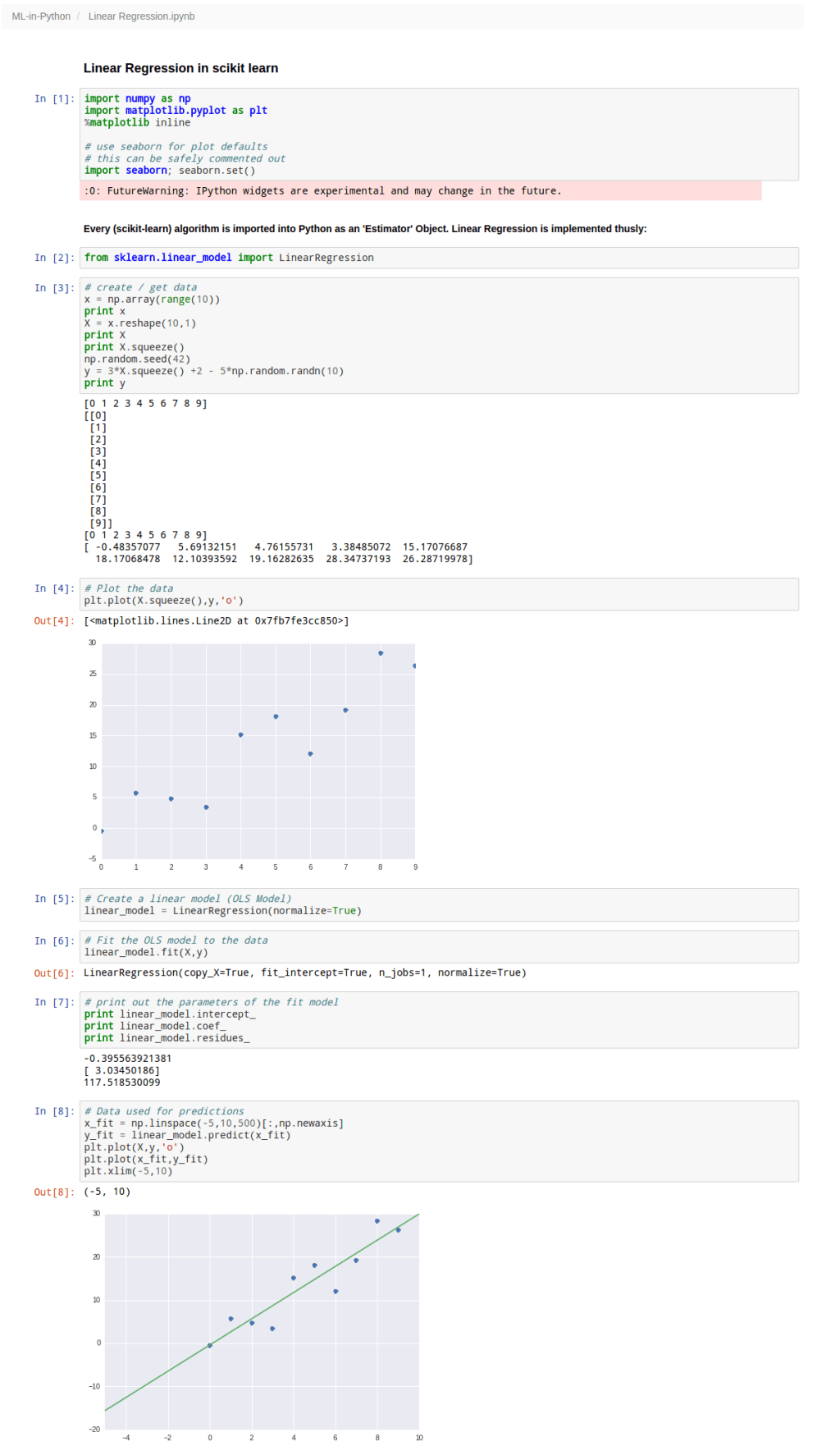
Here’s a quick example case for implementing one of the simplest of learning algorithms in any machine learning toolbox – Linear Regression. You can download the IPython / Jupyter notebook here so as to play around with the code and try things out yourself.
I’m doing a series of posts on scikit-learn. Its documentation is vast, so unless you’re willing to search for a needle in a haystack, you’re better off NOT jumping into the documentation right away. Instead, knowing chunks of code that do the job might help.
Find the kth smallest element in an array without sorting.
That’s basically what this algorithm does. It piggybacks on the partition subroutine from the Quick Sort. If you don’t know what that is, you can check out more about the Quick Sort algorithm here and here, and understand the usefulness of partitioning an unsorted array around a pivot.
Animated visualization of the randomized selection algorithm selecting the 22nd smallest value
Python Implementation
This file contains hidden or bidirectional Unicode text that may be interpreted or compiled differently than what appears below. To review, open the file in an editor that reveals hidden Unicode characters.
Learn more about bidirectional Unicode characters
A key aspect of the Quick Sort algorithm is how the pivot element is chosen. In my earlier post on the Python code for Quick Sort, my implementation takes the first element of the unsorted array as the pivot element.
However with some mathematical analysis it can be seen that such an implementation is O(n2) in complexity while if a pivot is randomly chosen, the Quick Sort algorithm is O(nlog2n).
To witness this in action, one can measure the work done by the algorithm comparing two cases, one with a randomized pivot choice – and one with a fixed pivot choice, say the first element of the array (or the last element of the array).
Implementation
A decent proxy for the amount of work done by the algorithm would be the number of pivot comparisons. These comparisons needn’t be computed one-by-one, rather when there is a recursive call on a subarray of length m, you should simply add m−1 to your running total of comparisons.
3 Cases
To put things in perspective, let’s look at 3 cases. (This is basically straight out of a homework assignment from Tim Roughgarden’s course on the Design and Analysis of Algorithms). Case I with the pivot being the first element. Case II with the pivot being the last element. Case III using the “median-of-three” pivot rule. The primary motivation behind this rule is to do a little bit of extra work to get much better performance on input arrays that are nearly sorted or reverse sorted.
Median-of-Three Pivot Rule
Consider the first, middle, and final elements of the given array. (If the array has odd length it should be clear what the “middle” element is; for an array with even length 2k, use the kth element as the “middle” element. So for the array 4 5 6 7, the “middle” element is the second one —- 5 and not 6! Identify which of these three elements is the median (i.e., the one whose value is in between the other two), and use this as your pivot.
This file contains all of the integers between 1 and 10,000 (inclusive, with no repeats) in unsorted order. The integer in the ith row of the file gives you the ith entry of an input array. I downloaded this file and named it QuickSort_List.txt
You can run the code below and see for yourself that the number of comparisons for Case III are 138,382 compared to 162,085 and 164,123 for Case I and Case II respectively. You can play around with the code in an IPython / Jupyter notebook here.
This file contains hidden or bidirectional Unicode text that may be interpreted or compiled differently than what appears below. To review, open the file in an editor that reveals hidden Unicode characters.
Learn more about bidirectional Unicode characters
Yet another post for the crawlers to better index my site for algorithms and as a repository for Python code. The quick sort algorithm is well explained in the topmost Google search result for ‘Quick Sort Python Code’, but the code is unnecessarily convoluted. Instead, go with the code below.
In it, I assume the pivot to be the first element. You can easily add a function to randomize selection of the pivot. Choosing a random pivot minimizes the chance that you will encounter worst-case O(n2) performance. Always choosing first or last would cause worst-case performance for nearly-sorted or nearly-reverse-sorted data.
This file contains hidden or bidirectional Unicode text that may be interpreted or compiled differently than what appears below. To review, open the file in an editor that reveals hidden Unicode characters.
Learn more about bidirectional Unicode characters