This is a very short post that will be very useful to help you quickly set up your COVID-19 datasets. I’m sharing code at the end of this post that scrapes through all CSV datasets made available by COVID19-India API.
We have exposed all the crowdsourced patient details, travel history (published by authorities) and statewise trends in this live API : https://t.co/tNyhpPYTJD A shout-out to all Data Analysts, Planners and Enthusiasts to use this data for helping the containment efforts. @_mekin
Copy paste this standalone script into your R environment and get going!
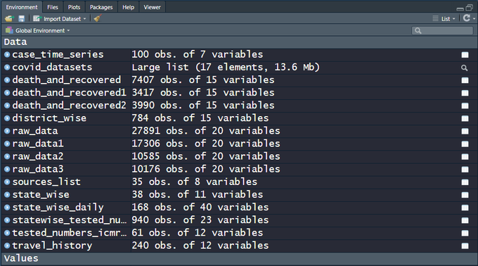
There are 15+ CSV files on the India COVID-19 API website. raw_data3 is actually a live dataset and more can be expected in the days to come, which is why a script that automates the data sourcing comes in handy. Snapshot of the file names and the data dimensions as of today, 100 days since the first case was recorded in the state of Kerala —
My own analysis of the data and predictions are work-in-progress, going into a Github repo. Execute the code below and get started analyzing the data and fighting COVID-19!
This file contains hidden or bidirectional Unicode text that may be interpreted or compiled differently than what appears below. To review, open the file in an editor that reveals hidden Unicode characters.
Learn more about bidirectional Unicode characters
The most conventional approach to determine structural breaks in longitudinal data seems to be the Chow Test.
From Wikipedia,
The Chow test, proposed by econometrician Gregory Chow in 1960, is a test of whether the coefficients in two linear regressions on different data sets are equal. In econometrics, it is most commonly used in time series analysis to test for the presence of a structural break at a period which can be assumed to be known a priori (for instance, a major historical event such as a war). In program evaluation, the Chow test is often used to determine whether the independent variables have different impacts on different subgroups of the population.
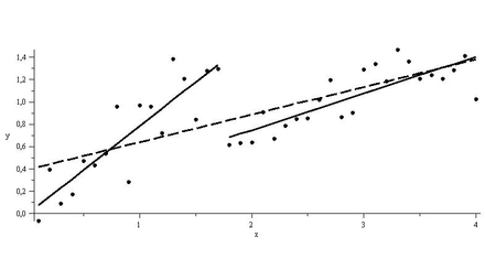
As shown in the figure below, regressions on the 2 sub-intervals seem to have greater explanatory power than a single regression over the data.
For the data above, determining the sub-intervals is an easy task. However, things may not look that simple in reality. Conducting a Chow test for structural breaks leaves the data scientist at the mercy of his subjective gaze in choosing a null hypothesis for a break point in the data.
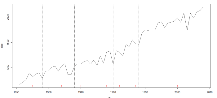
Instead of choosing the breakpoints in an exogenous manner, what if the data itself could learn where these breakpoints lie? Such an endogenous technique is what Bai and Perron came up with in a seminal paper published in 1998 that could detect multiple structural breaks in longitudinal data. A later paper in 2003 dealt with the testing for breaks empirically, using a dynamic programming algorithm based on the Bellmanprinciple.
I will discuss a quick implementation of this technique in R.
Brief Outline:
Assuming you have a ts object (I don’t know whether this works with zoo, but it should) in R, called ts. Then implement the following:
This file contains hidden or bidirectional Unicode text that may be interpreted or compiled differently than what appears below. To review, open the file in an editor that reveals hidden Unicode characters.
Learn more about bidirectional Unicode characters
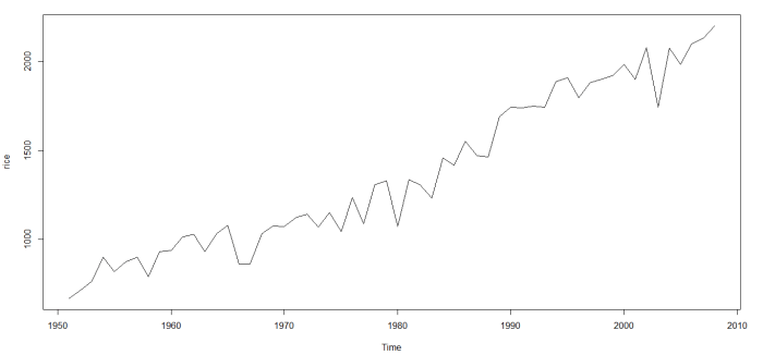
I started with data on India’s rice crop productivity between 1950 (around Independence from British Colonial rule) and 2008. Here’s how it looks:
You can download the excel and CSV files here and here respectively.
Here’s the way to go using R:
This file contains hidden or bidirectional Unicode text that may be interpreted or compiled differently than what appears below. To review, open the file in an editor that reveals hidden Unicode characters.
Learn more about bidirectional Unicode characters
Here’s a quick example case for implementing one of the simplest of learning algorithms in any machine learning toolbox – Linear Regression. You can download the IPython / Jupyter notebook here so as to play around with the code and try things out yourself.
I’m doing a series of posts on scikit-learn. Its documentation is vast, so unless you’re willing to search for a needle in a haystack, you’re better off NOT jumping into the documentation right away. Instead, knowing chunks of code that do the job might help.
This happens to be my 50th blog post – and my blog is 8 months old.
🙂
This post is the third and last post in in a series of posts (Part 1 – Part 2) on data manipulation with dlpyr. Note that the objects in the code may have been defined in earlier posts and the code in this post is in continuation with code from the earlier posts.
Although datasets can be manipulated in sophisticated ways by linking the 5 verbs of dplyr in conjunction, linking verbs together can be a bit verbose.
Creating multiple objects, especially when working on a large dataset can slow you down in your analysis. Chaining functions directly together into one line of code is difficult to read. This is sometimes called the Dagwood sandwich problem: you have too much filling (too many long arguments) between your slices of bread (parentheses). Functions and arguments get further and further apart.
The %>% operator allows you to extract the first argument of a function from the arguments list and put it in front of it, thus solving the Dagwood sandwich problem.
This file contains hidden or bidirectional Unicode text that may be interpreted or compiled differently than what appears below. To review, open the file in an editor that reveals hidden Unicode characters.
Learn more about bidirectional Unicode characters
group_by() defines groups within a data set. Its influence becomes clear when calling summarise() on a grouped dataset. Summarizing statistics are calculated for the different groups separately.
This file contains hidden or bidirectional Unicode text that may be interpreted or compiled differently than what appears below. To review, open the file in an editor that reveals hidden Unicode characters.
Learn more about bidirectional Unicode characters
group_by() can also be combined with mutate(). When you mutate grouped data, mutate() will calculate the new variables independently for each group. This is particularly useful when mutate() uses the rank() function, that calculates within group rankings. rank() takes a group of values and calculates the rank of each value within the group, e.g.
rank(c(21, 22, 24, 23))
has output
[1] 1 2 4 3
As with arrange(), rank() ranks values from the largest to the smallest and this behaviour can be reversed with the desc() function.
This file contains hidden or bidirectional Unicode text that may be interpreted or compiled differently than what appears below. To review, open the file in an editor that reveals hidden Unicode characters.
Learn more about bidirectional Unicode characters
On January 12, 2016, Stanford University professors Trevor Hastie and Rob Tibshirani will offer the 3rd iteration of Statistical Learning, a MOOC which first began in January 2014, and has become quite a popular course among data scientists. It is a great place to learn statistical learning (machine learning) methods using the R programming language. For a quick course on R, check this out – Introduction to R Programming
Slides and videos for Statistical Learning MOOC by Hastie and Tibshirani available separately here. Slides and video tutorials related to this book by Abass Al Sharif can be downloaded here.
The course covers the following book which is available for free as a PDF copy.
Logistics and Effort:
Rough Outline of Schedule (based on last year’s course offering):
Week 1: Introduction and Overview of Statistical Learning (Chapters 1-2) Week 2: Linear Regression (Chapter 3) Week 3: Classification (Chapter 4) Week 4: Resampling Methods (Chapter 5) Week 5: Linear Model Selection and Regularization (Chapter 6) Week 6: Moving Beyond Linearity (Chapter 7) Week 7: Tree-based Methods (Chapter 8) Week 8: Support Vector Machines (Chapter 9) Week 9: Unsupervised Learning (Chapter 10)
Prerequisites: First courses in statistics, linear algebra, and computing.
I found myself stuck on this problem recently. I must confess, I lost a couple of hours trying to get to figure the logic for this one. Here’s the problem:
I’ve written 2 functions to solve this problem. The first one I used for smaller N, say N < 30 and the second one for N > 30. The second function is elegant, and it relies on the mathematical property that if a number N is not divisible by 3, it could either leave a remainder 1 or 2.
If it leaves a remainder 2, then subtracting 5 once would make the number divisible by 3. If it leaves a remainder 1, then subtracting 5 twice would make the number divisible by 3.
We subtract 5 from N iteratively and attempt to divide N into 2 parts, one divisible by 3 and the other divisible by 5. We want the part that is divisible by 3 to be the larger part, so that the associated Decent Number is the largest possible. This explanation might seem obtuse, but if you get pen down on paper, you’ll understand what I mean.
This post contains links to a bunch of code that I have written to complete Andrew Ng’s famous machine learning course which includes several interesting machine learning problems that needed to be solved using the Octave / Matlab programming language. I’m not sure I’d ever be programming in Octave after this course, but learning Octave just so that I could complete this course seemed worth the time and effort. I would usually work on the programming assignments on Sundays and spend several hours coding in Octave, telling myself that I would later replicate the exercises in Python.
If you’ve taken this course and found some of the assignments hard to complete, I think it might not hurt to go check online on how a particular function was implemented. If you end up copying the entire code, it’s probably your loss in the long run. But then John Maynard Keynes once said, ‘In the long run we are all dead‘. Yeah, and we wonder why people call Economics the dismal science!
Most people disregard Coursera’s feeble attempt at reigning in plagiarism by creating an Honor Code, precisely because this so-called code-of-conduct can be easily circumvented. I don’t mind posting solutions to a course’s programming assignments because GitHub is full to the brim with such content. Plus, it’s always good to read others’ code even if you implemented a function correctly. It helps understand the different ways of tackling a given programming problem.
MIT’s Fall 2015 iteration of 6.00.2xstarts today. After an enriching learning experience with 6.00.1x, I have great expectations from this course. As the course website mildly puts it, 6.00.2x is an introduction to using computation to understand real-world phenomena. MIT OpenCourseware (OCW) mirroring the material covered in 6.00.1x and 6.00.2x can be found here.
The course follows this book by John Guttag (who happens to be one of the instructors for this course). However, purchasing the book isn’t a necessity for this course.
One thing I loved about 6.00.1x was its dedicated Facebook group, which gave a community / classroom-peergroup feel to the course. 6.00.2x also has a Facebook group. Here’s a sneak peak:
Thesyllabus and schedule for this course is shown below. The course is spread out over 2 months which includes 7 weeks of lectures.
MITx 6.00.2x Fall 2015 Course Calendar
The prerequisites for this course are pretty much covered in this set of tutorial videos that have been created by one of the TAs for 6.00.1x. If you’ve not taken 6.00.1x in the past, you can go through these videos (running time < 1hr) to judge whether or not to go ahead with 6.00.2x.
Programming as a profession is only moderately interesting. It can be a good job, but you could make about the same money and be happier running a fast food joint. You’re much better off using code as your secret weapon in another profession.
People who can code in the world of technology companies are a dime a dozen and get no respect. People who can code in biology, medicine, government, sociology, physics, history, and mathematics are respected and can do amazing things to advance those disciplines.
I was reading a paper today, written by MIT’s Esther Duflo, part of a homework assignment on a MOOC on development policy (Foundations of Development Policy: Advanced Development Economics) offered by Duflo and Abhijit Banerjee. So I opened the paper and started copying important lines from the PDF to a text editor to make notes. I could copy the text, but when I pasted it onto a text editor, it turned out to be gibberish (you can try it too!).
For instance, instead of pasting
Between 1973 and 1978 the Indonesian Government constructed over 61,000 primaryschools throughout the county
It was a good thing the cipher used for this text wasn’t too complicated. After some perusal, I found that ‘B’ became ‘E’, ‘e’ became ‘h’, ‘t’ became ‘w’ and so on. So I copied the entire content of the PDF to a text file and named the encrypted file estherDuflo.txt. I noticed that the encryption had been implemented only on the first 1475 lines. The remaining was plain English.
So I wrote a Python script to decrypt the gibberish, rather than simply typing out my notes. It took 20 minutes writing the code and 8 ms to execute (of course!). I didn’t want to spend a lot of time ensuring a thorough decryption, so the result wasn’t perfect, but then I’m going to make do. I named the decrypted file estherDufloDecrypted.txt.
This file contains hidden or bidirectional Unicode text that may be interpreted or compiled differently than what appears below. To review, open the file in an editor that reveals hidden Unicode characters.
Learn more about bidirectional Unicode characters
This file contains hidden or bidirectional Unicode text that may be interpreted or compiled differently than what appears below. To review, open the file in an editor that reveals hidden Unicode characters.
Learn more about bidirectional Unicode characters
This file contains hidden or bidirectional Unicode text that may be interpreted or compiled differently than what appears below. To review, open the file in an editor that reveals hidden Unicode characters.
Learn more about bidirectional Unicode characters
Yet another exciting math problem that requires an algorithmic approach to arrive at a quick solution! There is a pen-paper approach to it too, but this post assumes we’re more interested in discussing the programming angle.
Working clockwise, and starting from the group of three with the numerically lowest external node (4,3,2 in this example), each solution can be described uniquely. For example, the above solution can be described by the set: 4,3,2; 6,2,1; 5,1,3.
It is possible to complete the ring with four different totals: 9, 10, 11, and 12. There are eight solutions in total.
Total Solution Set: 9 4,2,3; 5,3,1; 6,1,2 9 4,3,2; 6,2,1; 5,1,3 10 2,3,5; 4,5,1; 6,1,3 10 2,5,3; 6,3,1; 4,1,5 11 1,4,6; 3,6,2; 5,2,4 11 1,6,4; 5,4,2; 3,2,6 12 1,5,6; 2,6,4; 3,4,5 12 1,6,5; 3,5,4; 2,4,6
By concatenating each group it is possible to form 9-digit strings; the maximum string for a 3-gon ring is432621513.
Problem
Using the numbers 1 to 10, and depending on arrangements, it is possible to form 16-and 17-digit strings. What is the maximum 16-digit string for a “magic” 5-gon ring?
Algorithm
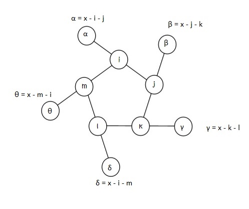
In attempting this problem, I choose to label the 5 inner nodes as i, j, k, l, and m. α, β, γ, δ, and θ being the corresponding outer nodes.
Let x be the sum total of each triplet line, i.e.,
x = α + i + j = β + j + k = γ + k + l = δ + l + m = θ + m + i
First Observation:
For the string to be 16-digits, 10 has to be in the outer ring, as each number in the inner ring is included in the string twice. Next, we fill the inner ring in an iterative manner.
Second Observation:
There 9 numbers to choose from for the inner ring — 1, 2, 3, 4, 5, 6, 7, 8 and 9.
5 have to be chosen. This can be done in 9C5 = 126 ways.
According to circular permutation, if there are n distinct numbers to be arranged in a circle, this can be done in (n-1)! ways, where (n-1)!= (n-1).(n-2).(n-3)…3.2.1. So 5 distinct numbers can be arranged in 4! permutations, i.e., in 24 ways around a circle, or pentagonal ring, to be more precise.
So in all, this problem can be solved in 126×24 =3024 iterations.
Third Observation:
For every possible permutation of an inner-ring arrangement, there can be one or more values of x(triplet line-sum) that serve as a possible contenders for a “magic”string whose triplets add up to the same number, x. To ensure this, we only need that the values of αthroughθ of the outer ring are distinct, different from the inner ring, with the greatest of these equal to 10.
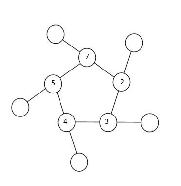
Depending on the relative positioning of the numbers in the inner ring, one can narrow the range of x-values one might have to check for each permutation. To zero-down on such a range, let’s look at an example. Shown in the figure below is a randomly chosen permutation of number in the inner ring – 7, 2, 3, 4 and 5, in that order.
So 10, 9, 8, 6 and 1 must fill the outer circle. It’s easy to notice that the 5, 7 pair is the greatest adjacent pair. So whatever x is, it has to be at least5 + 7 + 1 = 13 (1 being the smallest number of the outer ring). Likewise, 2, 3 is the smallest adjacent pair, so whatever x is, it can’t be any more than 2 + 3+ 10 = 15 (10 being the largest number of the outer ring). This leaves us with a narrow range of x-values to check – 13, 14 and 15.
Next, we arrange the 5 triplets in clock-wise direction starting with the triplet with the smallest number in the outer ring to form a candidate string. This exercise when done for each of the 3024permutations will shortlist a range of candidates, of which, the maximum is chosen.
That’s all there is to the problem!
Here’s the Python Code. It executes in about a tenth of a second!
This file contains hidden or bidirectional Unicode text that may be interpreted or compiled differently than what appears below. To review, open the file in an editor that reveals hidden Unicode characters.
Learn more about bidirectional Unicode characters