This post comes out of the blue, nearly 2 years since my last one. I realize I’ve been lazy, so here’s hoping I move from an inertia of rest to that of motion, implying, regular and (hopefully) relevant posts. I also chanced upon some wisdom while scrolling through my Twitter feed:
https://twitter.com/CoralineAda/status/1193216045210906625
This blog post in particular was meant to be a reminder to myself and other R users that the much used lm() function in R (for fitting linear models) can be replaced with some handy matrix operations to obtain regression coefficients, their standard errors and other goodness-of-fit stats printed out when summary() is called on an lm object.
Linear regression can be formulated mathematically as follows:


The covariance matrix can be obtained with some handy matrix operations:
given that


The standard errors of the coefficients are basically 
Lastly, the F-statistic and its corresponding p-value can be calculated after computing the two residual sum of squares (RSS) statistics:
– for the full model with all predictors
– for the partial model (
) with the outcome observed mean as estimated outcome

I wrote some R code to construct the output from summarizing lm objects, using all the math spewed thus far. The data used for this exercise is available in R, and comprises of standardized fertility measures and socio-economic indicators for each of 47 French-speaking provinces of Switzerland from 1888. Try it out and see for yourself the linear algebra behind linear regression.
| ### Linear Regression Using lm() —————————————- | |
| data("swiss") | |
| dat <- swiss | |
| linear_model <- lm(Fertility ~ ., data = dat) | |
| summary(linear_model) | |
| # Call: | |
| # lm(formula = Fertility ~ ., data = dat) | |
| # | |
| # Residuals: | |
| # Min 1Q Median 3Q Max | |
| # -15.2743 -5.2617 0.5032 4.1198 15.3213 | |
| # | |
| # Coefficients: | |
| # Estimate Std. Error t value Pr(>|t|) | |
| # (Intercept) 66.91518 10.70604 6.250 1.91e-07 *** | |
| # Agriculture -0.17211 0.07030 -2.448 0.01873 * | |
| # Examination -0.25801 0.25388 -1.016 0.31546 | |
| # Education -0.87094 0.18303 -4.758 2.43e-05 *** | |
| # Catholic 0.10412 0.03526 2.953 0.00519 ** | |
| # Infant.Mortality 1.07705 0.38172 2.822 0.00734 ** | |
| # — | |
| # Signif. codes: 0 ‘***’ 0.001 ‘**’ 0.01 ‘*’ 0.05 ‘.’ 0.1 ‘ ’ 1 | |
| # | |
| # Residual standard error: 7.165 on 41 degrees of freedom | |
| # Multiple R-squared: 0.7067, Adjusted R-squared: 0.671 | |
| # F-statistic: 19.76 on 5 and 41 DF, p-value: 5.594e-10 | |
| ### Using Linear Algebra ———————————————— | |
| y <- matrix(dat$Fertility, nrow = nrow(dat)) | |
| X <- cbind(1, as.matrix(x = dat[,-1])) | |
| colnames(X)[1] <- "(Intercept)" | |
| # N x k matrix | |
| N <- nrow(X) | |
| k <- ncol(X) – 1 # number of predictor variables (ergo, excluding Intercept column) | |
| # Estimated Regression Coefficients | |
| beta_hat <- solve(t(X)%*%X)%*%(t(X)%*%y) | |
| # Variance of outcome variable = Variance of residuals | |
| sigma_sq <- residual_variance <- (N-k-1)^-1 * sum((y – X %*% beta_hat)^2) | |
| residual_std_error <- sqrt(residual_variance) | |
| # Variance and Std. Error of estimated coefficients of the linear model | |
| var_betaHat <- sigma_sq * solve(t(X) %*% X) | |
| coeff_std_errors <- sqrt(diag(var_betaHat)) | |
| # t values of estimates are ratio of estimated coefficients to std. errors | |
| t_values <- beta_hat / coeff_std_errors | |
| # p-values of t-statistics of estimated coefficeints | |
| p_values_tstat <- 2 * pt(abs(t_values), N-k, lower.tail = FALSE) | |
| # assigning R's significance codes to obtained p-values | |
| signif_codes_match <- function(x){ | |
| ifelse(x <= 0.001,"***", | |
| ifelse(x <= 0.01,"**", | |
| ifelse(x < 0.05,"*", | |
| ifelse(x < 0.1,"."," ")))) | |
| } | |
| signif_codes <- sapply(p_values_tstat, signif_codes_match) | |
| # R-squared and Adjusted R-squared (refer any econometrics / statistics textbook) | |
| R_sq <- 1 – (N-k-1)*residual_variance / (N*mean((y – mean(y))^2)) | |
| R_sq_adj <- 1 – residual_variance / ((N/(N-1))*mean((y – mean(y))^2)) | |
| # Residual sum of squares (RSS) for the full model | |
| RSS <- (N-k-1)*residual_variance | |
| # RSS for the partial model with only intercept (equal to mean), ergo, TSS | |
| RSS0 <- TSS <- sum((y – mean(y))^2) | |
| # F statistic based on RSS for full and partial models | |
| # k = degress of freedom of partial model | |
| # N – k – 1 = degress of freedom of full model | |
| F_stat <- ((RSS0 – RSS)/k) / (RSS/(N-k-1)) | |
| # p-values of the F statistic | |
| p_value_F_stat <- pf(F_stat, df1 = k, df2 = N-k-1, lower.tail = FALSE) | |
| # stitch the main results toghether | |
| lm_results <- as.data.frame(cbind(beta_hat, coeff_std_errors, | |
| t_values, p_values_tstat, signif_codes)) | |
| colnames(lm_results) <- c("Estimate","Std. Error","t value","Pr(>|t|)","") | |
| ### Print out results of all relevant calcualtions ———————– | |
| print(lm_results) | |
| cat("Residual standard error: ", | |
| round(residual_std_error, digits = 3), | |
| " on ",N-k-1," degrees of freedom", | |
| "\nMultiple R-squared: ",R_sq," Adjusted R-squared: ",R_sq_adj, | |
| "\nF-statistic: ",F_stat, " on ",k-1," and ",N-k-1, | |
| " DF, p-value: ", p_value_F_stat,"\n") | |
| # Estimate Std. Error t value Pr(>|t|) | |
| # (Intercept) 66.9151816789654 10.7060375853301 6.25022854119771 1.73336561301153e-07 *** | |
| # Agriculture -0.172113970941457 0.0703039231786469 -2.44814177018405 0.0186186100433133 * | |
| # Examination -0.258008239834722 0.253878200892098 -1.01626779663678 0.315320687313066 | |
| # Education -0.870940062939429 0.183028601571259 -4.75849159892283 2.3228265226988e-05 *** | |
| # Catholic 0.104115330743766 0.035257852536169 2.95296858017545 0.00513556154915653 ** | |
| # Infant.Mortality 1.07704814069103 0.381719650858061 2.82156849475775 0.00726899472564356 ** | |
| # Residual standard error: 7.165 on 41 degrees of freedom | |
| # Multiple R-squared: 0.706735 Adjusted R-squared: 0.670971 | |
| # F-statistic: 19.76106 on 4 and 41 DF, p-value: 5.593799e-10 | |
Hope this was useful and worth your time!


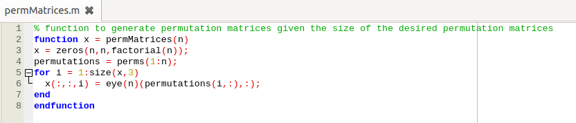
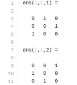
 To solve this quickly, it would have been nice to have a function that would give a list of permutation matrices for every n-sized square matrix, but there was none in Octave, so I wrote a function
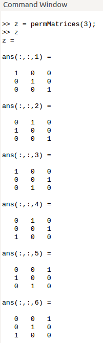


 single-digit multiplications in general (and exactly
  when n is a power of 2). Although the familiar grade school algorithm for multiplying numbers is how we work through multiplication in our day-to-day lives, it’s slower (
 ) in comparison, but only on a computer, of course!


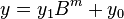
 and
and  be represented as
  -digit strings in some
  . For any positive integer
  less than
 ,
, and
and  are less than
  . The product is then
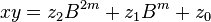


 can be computed in only three multiplications, at the cost of a few extra additions. With
  and
and  as before we can calculate

 , where
  .
.