Linear Algebra behind the lm() function in R

This post comes out of the blue, nearly 2 years since my last one. I realize I’ve been lazy, so here’s hoping I move from an inertia of rest to that of motion, implying, regular and (hopefully) relevant posts. I also chanced upon some wisdom while scrolling through my Twitter feed:

This blog post in particular was meant to be a reminder to myself and other R users that the much used lm() function in R (for fitting linear models) can be replaced with some handy matrix operations to obtain regression coefficients, their standard errors and other goodness-of-fit stats printed out when summary() is called on an lm object.

Linear regression can be formulated mathematically as follows:
\mathbf{y} = \mathbf{X} \mathbf{\beta} + \mathbf{\epsilon} ,
\mathbf{\epsilon} \sim N(0, \sigma^2 \mathbf{I})

\mathbf{y} is the \mathbf{n}\times \mathbf{1} outcome variable and \mathbf{X} is the \mathbf{n}\times \mathbf{(\mathbf{k}+1)} data matrix of independent predictor variables (including a vector of ones corresponding to the intercept). The ordinary least squares (OLS) estimate for the vector of coefficients \mathbf{\beta} is:

\hat{\mathbf{\beta}} = (\mathbf{X}^{\prime} \mathbf{X})^{-1} \mathbf{X}^{\prime} \mathbf{y}

The covariance matrix can be obtained with some handy matrix operations:
\textrm{Var}(\hat{\mathbf{\beta}}) = (\mathbf{X}^{\prime} \mathbf{X})^{-1} \mathbf{X}^{\prime} \;\sigma^2 \mathbf{I} \; \mathbf{X} (\mathbf{X}^{\prime} \mathbf{X})^{-1} = \sigma^2 (\mathbf{X}^{\prime} \mathbf{X})^{-1}
given that \textrm{Var}(AX) = A \times \textrm{Var}X \times A^{\prime}; \textrm{Var}(\mathbf{y}) = \mathbf{\sigma^2}

The standard errors of the coefficients are basically \textrm{Diag}(\sqrt{\textrm{Var}(\hat{\mathbf{\beta}})}) = \textrm{Diag}(\sqrt{\sigma^2 (\mathbf{X}^{\prime} \mathbf{X})^{-1}}) and with these, one can compute the t-statistics and their corresponding p-values.

Lastly, the F-statistic and its corresponding p-value can be calculated after computing the two residual sum of squares (RSS) statistics:

  • \mathbf{RSS} – for the full model with all predictors
  • \mathbf{RSS_0} – for the partial model (\mathbf{y} = \mathbf{\mu} + \mathbf{\nu}; \mathbf{\mu} = \mathop{\mathbb{E}}[\mathbf{y}]; \mathbf{\nu} \sim N(0, \sigma_0^2 \mathbf{I}) ) with the outcome observed mean as estimated outcome

\mathbf{F} = \frac{(\mathbf{RSS_0}-\mathbf{RSS})/\mathbf{k}}{\mathbf{RSS}/(\mathbf{n}-\mathbf{k}-1)}

I wrote some R code to construct the output from summarizing lm objects, using all the math spewed thus far. The data used for this exercise is available in R, and comprises of standardized fertility measures and socio-economic indicators for each of 47 French-speaking provinces of Switzerland from 1888. Try it out and see for yourself the linear algebra behind linear regression.

### Linear Regression Using lm() ----------------------------------------
data("swiss")
dat <- swiss
linear_model <- lm(Fertility ~ ., data = dat)
summary(linear_model)
# Call:
# lm(formula = Fertility ~ ., data = dat)
#
# Residuals:
# Min 1Q Median 3Q Max
# -15.2743 -5.2617 0.5032 4.1198 15.3213
#
# Coefficients:
# Estimate Std. Error t value Pr(>|t|)
# (Intercept) 66.91518 10.70604 6.250 1.91e-07 ***
# Agriculture -0.17211 0.07030 -2.448 0.01873 *
# Examination -0.25801 0.25388 -1.016 0.31546
# Education -0.87094 0.18303 -4.758 2.43e-05 ***
# Catholic 0.10412 0.03526 2.953 0.00519 **
# Infant.Mortality 1.07705 0.38172 2.822 0.00734 **
# ---
# Signif. codes: 0 ‘***’ 0.001 ‘**’ 0.01 ‘*’ 0.05 ‘.’ 0.1 ‘ ’ 1
#
# Residual standard error: 7.165 on 41 degrees of freedom
# Multiple R-squared: 0.7067, Adjusted R-squared: 0.671
# F-statistic: 19.76 on 5 and 41 DF, p-value: 5.594e-10
### Using Linear Algebra ------------------------------------------------
y <- matrix(dat$Fertility, nrow = nrow(dat))
X <- cbind(1, as.matrix(x = dat[,-1]))
colnames(X)[1] <- "(Intercept)"
# N x k matrix
N <- nrow(X)
k <- ncol(X) - 1 # number of predictor variables (ergo, excluding Intercept column)
# Estimated Regression Coefficients
beta_hat <- solve(t(X)%*%X)%*%(t(X)%*%y)
# Variance of outcome variable = Variance of residuals
sigma_sq <- residual_variance <- (N-k-1)^-1 * sum((y - X %*% beta_hat)^2)
residual_std_error <- sqrt(residual_variance)
# Variance and Std. Error of estimated coefficients of the linear model
var_betaHat <- sigma_sq * solve(t(X) %*% X)
coeff_std_errors <- sqrt(diag(var_betaHat))
# t values of estimates are ratio of estimated coefficients to std. errors
t_values <- beta_hat / coeff_std_errors
# p-values of t-statistics of estimated coefficeints
p_values_tstat <- 2 * pt(abs(t_values), N-k, lower.tail = FALSE)
# assigning R's significance codes to obtained p-values
signif_codes_match <- function(x){
ifelse(x <= 0.001,"***",
ifelse(x <= 0.01,"**",
ifelse(x < 0.05,"*",
ifelse(x < 0.1,"."," "))))
}
signif_codes <- sapply(p_values_tstat, signif_codes_match)
# R-squared and Adjusted R-squared (refer any econometrics / statistics textbook)
R_sq <- 1 - (N-k-1)*residual_variance / (N*mean((y - mean(y))^2))
R_sq_adj <- 1 - residual_variance / ((N/(N-1))*mean((y - mean(y))^2))
# Residual sum of squares (RSS) for the full model
RSS <- (N-k-1)*residual_variance
# RSS for the partial model with only intercept (equal to mean), ergo, TSS
RSS0 <- TSS <- sum((y - mean(y))^2)
# F statistic based on RSS for full and partial models
# k = degress of freedom of partial model
# N - k - 1 = degress of freedom of full model
F_stat <- ((RSS0 - RSS)/k) / (RSS/(N-k-1))
# p-values of the F statistic
p_value_F_stat <- pf(F_stat, df1 = k, df2 = N-k-1, lower.tail = FALSE)
# stitch the main results toghether
lm_results <- as.data.frame(cbind(beta_hat, coeff_std_errors,
t_values, p_values_tstat, signif_codes))
colnames(lm_results) <- c("Estimate","Std. Error","t value","Pr(>|t|)","")
### Print out results of all relevant calcualtions -----------------------
print(lm_results)
cat("Residual standard error: ",
round(residual_std_error, digits = 3),
" on ",N-k-1," degrees of freedom",
"\nMultiple R-squared: ",R_sq," Adjusted R-squared: ",R_sq_adj,
"\nF-statistic: ",F_stat, " on ",k-1," and ",N-k-1,
" DF, p-value: ", p_value_F_stat,"\n")
# Estimate Std. Error t value Pr(>|t|)
# (Intercept) 66.9151816789654 10.7060375853301 6.25022854119771 1.73336561301153e-07 ***
# Agriculture -0.172113970941457 0.0703039231786469 -2.44814177018405 0.0186186100433133 *
# Examination -0.258008239834722 0.253878200892098 -1.01626779663678 0.315320687313066
# Education -0.870940062939429 0.183028601571259 -4.75849159892283 2.3228265226988e-05 ***
# Catholic 0.104115330743766 0.035257852536169 2.95296858017545 0.00513556154915653 **
# Infant.Mortality 1.07704814069103 0.381719650858061 2.82156849475775 0.00726899472564356 **
# Residual standard error: 7.165 on 41 degrees of freedom
# Multiple R-squared: 0.706735 Adjusted R-squared: 0.670971
# F-statistic: 19.76106 on 4 and 41 DF, p-value: 5.593799e-10

Hope this was useful and worth your time!
Advertisement

Endogenously Detecting Structural Breaks in a Time Series: Implementation in R

The most conventional approach to determine structural breaks in longitudinal data seems to be the Chow Test.

From Wikipedia,

The Chow test, proposed by econometrician Gregory Chow in 1960, is a test of whether the coefficients in two linear regressions on different data sets are equal. In econometrics, it is most commonly used in time series analysis to test for the presence of a structural break at a period which can be assumed to be known a priori (for instance, a major historical event such as a war). In program evaluation, the Chow test is often used to determine whether the independent variables have different impacts on different subgroups of the population.

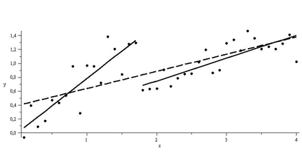
As shown in the figure below, regressions on the 2 sub-intervals seem to have greater explanatory power than a single regression over the data.

440px-chow_test_structural_break

For the data above, determining the sub-intervals is an easy task. However, things may not look that simple in reality. Conducting a Chow test for structural breaks leaves the data scientist at the mercy of his subjective gaze in choosing a null hypothesis for a break point in the data.

Instead of choosing the breakpoints in an exogenous manner, what if the data itself could learn where these breakpoints lie? Such an endogenous technique is what Bai and Perron came up with in a seminal paper published in 1998 that could detect multiple structural breaks in longitudinal data. A later paper in 2003 dealt with the testing for breaks empirically, using a dynamic programming algorithm based on the Bellman principle.

I will discuss a quick implementation of this technique in R.

Brief Outline:

Assuming you have a ts object (I don’t know whether this works with zoo, but it should) in R, called ts. Then implement the following:

# assuming you have a 'ts' object in R
# 1. install package 'strucchange'
# 2. Then write down this code:
library(strucchange)
# store the breakdates
bp_ts <- breakpoints(ts ~ 1)
# this will give you the break dates and their confidence intervals
summary(bp_ts)
# store the confidence intervals
ci_ts <- confint(bp_ts)
## to plot the breakpoints with confidence intervals
plot(ts)
lines(bp_ts)
lines(ci_ts)

An illustration 

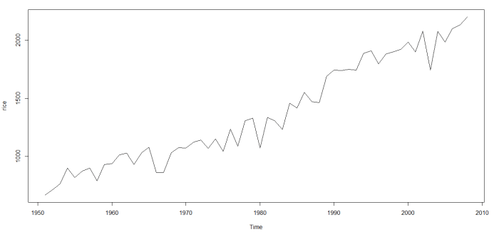
I started with data on India’s rice crop productivity between 1950 (around Independence from British Colonial rule) and 2008. Here’s how it looks:

rice_productivity

You can download the excel and CSV files here and here respectively.

Here’s the way to go using R:

library(xlsx)
library(forecast)
library(tseries)
library(strucchange)
## load the data from a CSV or Excel file. This example is done with an Excel sheet.
prod_df <- read.xlsx(file = 'agricultural_productivity.xls', sheetIndex = 'Sheet1', rowIndex = 8:65, colIndex = 2, header = FALSE)
colnames(prod_df) <- c('Rice')
## store rice data as time series objects
rice <- ts(prod_df$Rice, start=c(1951, 1), end=c(2008, 1), frequency=1)
# store the breakpoints
bp.rice <- breakpoints(rice ~ 1)
summary(bp.rice)
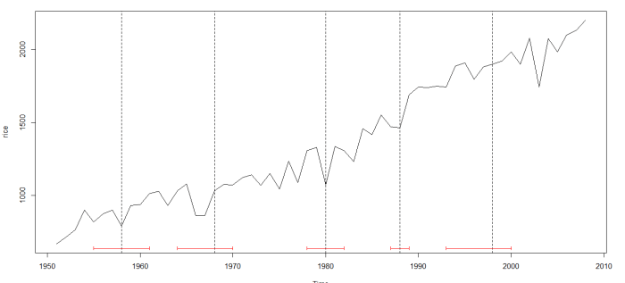
## the BIC chooses 5 breakpoints; plot the graph with breakdates and their confidence intervals
plot(bp.rice)
plot(rice)
lines(bp.rice)
## confidence intervals
ci.rice <- confint(bp.rice)
ci.rice
lines(ci.rice)

Voila, this is what you get:

02_rice_multiplebreaks

The dotted vertical lines indicated the break dates; the horizontal red lines indicate their confidence intervals.

This is a quick and dirty implementation. For a more detailed take, check out the documentation on the R package called strucchange.

Detecting Structural Breaks in China’s FX Regime

Edit: This post is in its infancy. Work is still ongoing as far as deriving insight from the data is concerned. More content and economic insight is expected to be added to this post as and when progress is made in that direction.

This is an attempt to detect structural breaks in China’s FX regime using Frenkel Wei regression methodology (this was later improved by Perron and Bai). I came up with the motivation to check for these structural breaks while attending a guest lecture on FX regimes by Dr. Ajay Shah delivered at IGIDR. This is work that I and two other classmates are working on as a term paper project under the supervision of Dr. Rajeswari Sengupta.

The code below can be replicated and run as is, to get same results.

## if fxregime or strucchange package is absent from installed packages, download it and load it
if(!require('fxregime')){
install.packages("fxregime")
}
if(!require('strucchange')){
install.packages("strucchange")
}
## load packages
library("fxregime")
library('strucchange')
# load the necessary data related to exchange rates - 'FXRatesCHF'
# this dataset treats CHF as unit currency
data("FXRatesCHF", package = "fxregime")
## compute returns for CNY (and explanatory currencies)
## since China abolished fixed USD regime
cny <- fxreturns("CNY", frequency = "daily",
start = as.Date("2005-07-25"), end = as.Date("2010-02-12"),
other = c("USD", "JPY", "EUR", "GBP"))
## compute all segmented regression with minimal segment size of
## h = 100 and maximal number of breaks = 10
regx <- fxregimes(CNY ~ USD + JPY + EUR + GBP,
data = cny, h = 100, breaks = 10, ic = "BIC")
## Print summary of regression results
summary(regx)
## minimum BIC is attained for 2-segment (1-break) model
plot(regx)
round(coef(regx), digits = 3)
sqrt(coef(regx)[, "(Variance)"])
## inspect associated confidence intervals
cit <- confint(regx, level = 0.9)
cit
breakdates(cit)
## plot LM statistics along with confidence interval
flm <- fxlm(CNY ~ USD + JPY + EUR + GBP, data = cny)
scus <- gefp(flm, fit = NULL)
plot(scus, functional = supLM(0.1))
## add lines related to breaks to your plot
lines(cit)

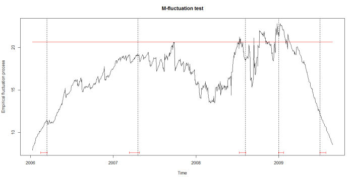
As can be seen in the figure below, the structural breaks correspond to the vertical bars. We are still working on understanding the motivations of China’s central bank in varying the degree of the managed float exchange rate.

strucchange_china_2006_2010

EDIT (May 16, 2016):

The code above uses data provided by the package itself. If you wished to replicate this analysis on data after 2010, you will have to use your own data. We used Quandl, which lets you get 10 premium datasets for free. An API key (for only 10 calls on premium datasets) is provided if you register there. Foreign exchange rate data (2000 onward till date) apparently, is premium data. You can find these here.

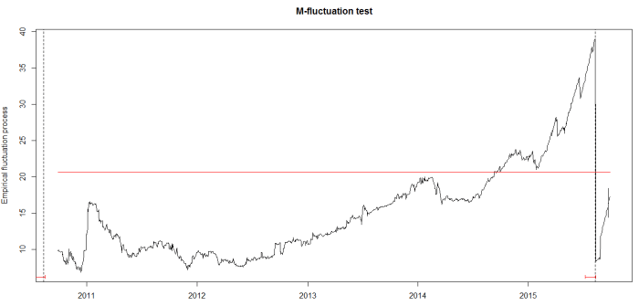
Here are the (partial) results and code to work the same methodology on the data from 2010 to 2016:

20102016

## if fxregime is absent from installed packages, download it and load it
if(!require('fxregime')){
install.packages("fxregime")
}
## load package
library("fxregime")
# load the necessary data related to exchange rates - 'FXRatesCHF'
# this dataset treats CHF as unit currency
# install / load Quandl
if(!require('Quandl')){
install.packages("Quandl")
}
library(Quandl)
# Extract and load currency data series with respect to CHF from Quandl
# Extract data series from Quandl. Each Quandl user will have unique api_key
# upon signing up. The freemium version allows access up to 10 fx rate data sets
# USDCHF <- Quandl("CUR/CHF", api_key="p2GsFxccPGFSw7n1-NF9")
# write.csv(USDCHF, file = "USDCHF.csv")
# USDCNY <- Quandl("CUR/CNY", api_key="p2GsFxccPGFSw7n1-NF9")
# write.csv(USDCNY, file = "USDCNY.csv")
# USDJPY <- Quandl("CUR/JPY", api_key="p2GsFxccPGFSw7n1-NF9")
# write.csv(USDJPY, file = "USDJPY.csv")
# USDEUR <- Quandl("CUR/EUR", api_key="p2GsFxccPGFSw7n1-NF9")
# write.csv(USDEUR, file = "USDEUR.csv")
# USDGBP <- Quandl("CUR/GBP", api_key="p2GsFxccPGFSw7n1-NF9")
# write.csv(USDGBP, file = "USDGBP.csv")
# load the data sets into R
USDCHF <- read.csv("G:/China's Economic Woes/USDCHF.csv")
USDCHF <- USDCHF[,2:3]
USDCNY <- read.csv("G:/China's Economic Woes/USDCNY.csv")
USDCNY <- USDCNY[,2:3]
USDEUR <- read.csv("G:/China's Economic Woes/USDEUR.csv")
USDEUR <- USDEUR[,2:3]
USDGBP <- read.csv("G:/China's Economic Woes/USDGBP.csv")
USDGBP <- USDGBP[,2:3]
USDJPY <- read.csv("G:/China's Economic Woes/USDJPY.csv")
USDJPY <- USDJPY[,2:3]
start = 1 # corresponds to 2016-05-12
end = 2272 # corresponds to 2010-02-12
dates <- as.Date(USDCHF[start:end,1])
USD <- 1/USDCHF[start:end,2]
CNY <- USDCNY[start:end,2]/USD
JPY <- USDJPY[start:end,2]/USD
EUR <- USDEUR[start:end,2]/USD
GBP <- USDGBP[start:end,2]/USD
# reverse the order of the vectors to reflect dates from 2005 - 2010 instead of
# the other way around
USD <- USD[length(USD):1]
CNY <- CNY[length(CNY):1]
JPY <- JPY[length(JPY):1]
EUR <- EUR[length(EUR):1]
GBP <- GBP[length(GBP):1]
dates <- dates[length(dates):1]
df <- data.frame(CNY, USD, JPY, EUR, GBP)
df$weekday <- weekdays(dates)
row.names(df) <- dates
df <- subset(df, weekday != 'Sunday')
df <- subset(df, weekday != 'Saturday')
df <- df[,1:5]
zoo_df <- as.zoo(df)
# Code to replicate analysis
cny_rep <- fxreturns("CNY", data = zoo_df, frequency = "daily",
other = c("USD", "JPY", "EUR", "GBP"))
time(cny_rep) <- as.Date(row.names(df)[2:1627])
regx_rep <- fxregimes(CNY ~ USD + JPY + EUR + GBP,
data = cny_rep, h = 100, breaks = 10, ic = "BIC")
summary(regx_rep)
## minimum BIC is attained for 2-segment (5-break) model
plot(regx_rep)
round(coef(regx_rep), digits = 3)
sqrt(coef(regx_rep)[, "(Variance)"])
## inspect associated confidence intervals
cit_rep <- confint(regx_rep, level = 0.9)
breakdates(cit_rep)
## plot LM statistics along with confidence interval
flm_rep <- fxlm(CNY ~ USD + JPY + EUR + GBP, data = cny_rep)
scus_rep <- gefp(flm_rep, fit = NULL)
plot(scus_rep, functional = supLM(0.1))
## add lines related to breaks to your plot
lines(cit_rep)
apply(cny_rep,1,function(x) sum(is.na(x)))

We got breaks in 2010 and in 2015 (when China’s stock markets crashed). We would have hoped for more breaks (we can still get them), but that would depend on the parameters chosen for our regression.


Python to the Rescue

Another journal-like entry

Programming as a profession is only moderately interesting. It can be a good job, but you could make about the same money and be happier running a fast food joint. You’re much better off using code as your secret weapon in another profession.

People who can code in the world of technology companies are a dime a dozen and get no respect. People who can code in biology, medicine, government, sociology, physics, history, and mathematics are respected and can do amazing things to advance those disciplines.

Advice from an Old Programmer

I was reading a paper today, written by MIT’s Esther Duflo, part of a homework assignment on a MOOC on development policy (Foundations of Development Policy: Advanced Development Economics) offered by Duflo and Abhijit Banerjee. So I opened the paper and started copying important lines from the PDF to a text editor to make notes. I could copy the text, but when I pasted it onto a text editor, it turned out to be gibberish (you can try it too!).

For instance, instead of pasting

Between 1973 and 1978 the Indonesian Government constructed over 61,000 primary schools throughout the county

I got:

Ehwzhhq 4<:6 dqg 4<:;/ wkh Lqgrqhvldq Jryhuqphqw frqv wuxfwhg ryhu 94/333 sulpdu| vfkrrov wkurxjkrxw wkh frxqwu|

It was a good thing the cipher used for this text wasn’t too complicated. After some perusal, I found that ‘B’ became ‘E’, ‘e’ became ‘h’, ‘t’ became ‘w’ and so on. So I copied the entire content of the PDF to a text file and named the encrypted file estherDuflo.txt. I noticed that the encryption had been implemented only on the first 1475 lines. The remaining was plain English.

So I wrote a Python script to decrypt the gibberish, rather than simply typing out my notes. It took 20 minutes writing the code and 8 ms to execute (of course!). I didn’t want to spend a lot of time ensuring a thorough decryption, so the result wasn’t perfect, but then I’m going to make do. I named the decrypted file estherDufloDecrypted.txt.

Sample from the Encrypted File

5U LL*?} @?_ w@MLh @h!i| L?ti^ i?Uit Lu 5U LL*
L?t|h U|L? ? W?_L?it@G ,_i?Ui uhL4 @? N? t @* L*U)
, Tih4i?|
,t| ih # L
W
Devwudfw
Ehwzhhq 4<:6 dqg 4<:;/ wkh Lqgrqhvldq Jryhuqphqw frqvwuxfwhg ryhu 94/333 sulpdu|
vfkrrov wkurxjkrxw wkh frxqwu|1 Wklv lv rqh ri wkh odujhvw vfkrro frqvwuxfwlrq surjudpv rq
uhfrug1 L hydoxdwh wkh hhfw ri wklv surjudp rq hgxfdwlrq dqg zdjhv e| frpelqlqj glhuhqfhv
dfurvv uhjlrqv lq wkh qxpehu ri vfkrrov frqvwuxfwhg zlwk glhuhqfhv dfurvv frkruwv lqgxfhg
e| wkh wlplqj ri wkh surjudp1 Wkh hvwlpdwhv vxjjhvw wkdw wkh frqvwuxfwlrq ri sulpdu| vfkrrov
ohg wr dq lqfuhdvh lq hgxfdwlrq dqg hduqlqjv1 Fkloguhq djhg 5 wr 9 lq 4<:7 uhfhlyhg 3145 wr
314< pruh |hduv ri hgxfdwlrq iru hdfk vfkrro frqvwuxfwhg shu 4/333 fkloguhq lq wkhlu uhjlrq
ri eluwk1 Xvlqj wkh yduldwlrqv lq vfkrrolqj jhqhudwhg e| wklv srolf| dv lqvwuxphqwdo yduldeohv
iru wkh lpsdfw ri hgxfdwlrq rq zdjhv jhqhudwhv hvwlpdwhv ri hfrqrplf uhwxuqv wr hgxfdwlrq
udqjlqj iurp 91; shufhqw wr 4319 shufhqw1 +MHO L5/ M64/ R48/ R55,
Wkh txhvwlrq ri zkhwkhu lqyhvwphqw lq lqiudvwuxfwxuh lqfuhdvhv kxpdq fdslwdo dqg uhgxfhv
sryhuw| kdv orqj ehhq d frqfhuq wr ghyhorsphqw hfrqrplvwv dqg srolf|pdnhuv1 Iru h{dpsoh/
dydlodelolw| ri vfkrrolqj lqiudvwuxfwxuh kdv ehhq vkrzq wr eh srvlwlyho| fruuhodwhg zlwk frpsohwhg
vfkrrolqj ru hquroophqw e| Qdqf| Elugvdoo +4<;8, lq xuedq Eud}lo/ Ghqqlv GhWud| +4<;;, dqg Ohh
view raw estherDuflo.txt hosted with ❤ by GitHub

My Code
from string import *
# create decipher dictionary
l = letters[:26]
decipher = "".join([l[(i+3)%26] for i in range(len(l))])
decipher = dict(zip(decipher,l))
# open and read encrypted text
filename = 'estherDuflo.txt'
f = open(filename, 'rw')
lines = f.readlines()
lines = [l[:-1] for l in lines]
# use first 1475 lines only
newlines = lines[:1475]
# apply decryption on those 1475 lines
decipheredLines = []
for line in newlines:
x = line.lower()
s = []
for letter in x:
if letter in letters:
s.append(decipher[letter])
else:
s.append(letter)
s.append('\n')
decipheredLines.append(''.join(s))
# write deciphered text to new text file
decipheredFile = 'estherDufloDeciphered.txt'
df = open(decipheredFile, 'w')
for line in decipheredLines:
df.write("%s" % line)
# close both text files
f.close()
df.close()
view raw estherDuflo.py hosted with ❤ by GitHub

Sample from the Decrypted File
5r ii*?} @?_ t@jie @e!f| i?qf^ f?rfq ir 5r ii*
i?q|e r|i? ? t?_i?fq@d ,_f?rf rei4 @? k? q @* i*r)
, qfe4f?|
,q| fe # i
t
abstract
between 4<:6 and 4<:;/ the indonesian government constructed over 94/333 primar|
schools throughout the countr|1 this is one of the largest school construction programs on
record1 i evaluate the eect of this program on education and wages b| combining dierences
across regions in the number of schools constructed with dierences across cohorts induced
b| the timing of the program1 the estimates suggest that the construction of primar| schools
led to an increase in education and earnings1 children aged 5 to 9 in 4<:7 received 3145 to
314< more |ears of education for each school constructed per 4/333 children in their region
of birth1 using the variations in schooling generated b| this polic| as instrumental variables
for the impact of education on wages generates estimates of economic returns to education
ranging from 91; percent to 4319 percent1 +jel i5/ j64/ o48/ o55,
the question of whether investment in infrastructure increases human capital and reduces
povert| has long been a concern to development economists and polic|makers1 for e{ample/
availabilit| of schooling infrastructure has been shown to be positivel| correlated with completed
schooling or enrollment b| nanc| birdsall +4<;8, in urban bra}il/ dennis detra| +4<;;, and lee

Getting Started with R on MIT’s 14.74x (Foundations of Development Policy)

I noticed that a major grievance of many students enrolled in MIT‘s latest edX course on development policy (Foundations of Development Policy: Advanced Development Economics) was that there wasn’t enough done to get them going with the R assignments. I have posted the R code for the homework (past the deadline, of course) of the first 2 weeks, so that others get a hang of the level of R that might be needed to solve these assignments in the following weeks. I’m willing to help out those needing help getting up to speed with R required for this course. For specific queries, leave your message in the comments section.

A great place to get spend time learning R before taking Foundations of Development Policy (14.74x) would be another edX course that’s been getting great reviews recently: Introduction to R Programming

R Code for Home Work (Week 1)

# set working directory to local directory where the data is kept
setwd("~/IGIDR/Development Economics - MIT/Homework Assignment 01")
# read the data
wb_dev_ind = read.csv("wb_dev_ind.csv")
# summarize data
summary(wb_dev_ind)
# Question 1
# What is the Mean of GDP per capita? What is the standard deviation of GDP per capita?
meanGDPperCapita = mean(wb_dev_ind$gdp_per_capita, na.rm = TRUE)
print(round(meanGDPperCapita))
sdGDPperCapita = sd(wb_dev_ind$gdp_per_capita, na.rm = TRUE)
print(round(sdGDPperCapita))
# Question 2
# What is the mean illiteracy rate across all countries? What is the standard deviation?
illiteracy_all = numeric(nrow(wb_dev_ind))
wb_dev_ind$illiteracy_all = illiteracy_all
wb_dev_ind$illiteracy_all = 100 - wb_dev_ind$literacy_all
meanIlliteracy = mean(wb_dev_ind$illiteracy_all, na.rm = TRUE)
print(round(meanIlliteracy))
sdIlliteracy = sd(wb_dev_ind$illiteracy_all, na.rm = TRUE)
print(round(sdIlliteracy))
# Question 3
# What is the mean infant mortality rate across all countries? What is the standard deviation?
meanInfantMortality = mean(wb_dev_ind$infant_mortality, na.rm = TRUE)
print(round(meanInfantMortality))
sdInfantMortality = sd(wb_dev_ind$infant_mortality, na.rm = TRUE)
print(round(sdInfantMortality))
# Question 4
# What is the mean male illiteracy rate? What is the mean female illiteracy rate?
illiteracy_male = numeric(nrow(wb_dev_ind))
wb_dev_ind$illiteracy_male = illiteracy_male
wb_dev_ind$illiteracy_male = 100 - wb_dev_ind$literacy_male
meanIlliteracyMale = mean(wb_dev_ind$illiteracy_male, na.rm = TRUE)
print(round(meanIlliteracyMale))
sdIlliteracyMale = sd(wb_dev_ind$illiteracy_male, na.rm = TRUE)
print(round(sdIlliteracyMale))
illiteracy_female = numeric(nrow(wb_dev_ind))
wb_dev_ind$illiteracy_female = illiteracy_female
wb_dev_ind$illiteracy_female = 100 - wb_dev_ind$literacy_female
meanIlliteracyFemale = mean(wb_dev_ind$illiteracy_female, na.rm = TRUE)
print(round(meanIlliteracyFemale))
sdIlliteracyFemale = sd(wb_dev_ind$illiteracy_female, na.rm = TRUE)
print(round(sdIlliteracyFemale))
# Question 5
# What are the mean, minimum, and maximum illiteracy rate among the 50 richest countries
richest50 = wb_dev_ind[order(wb_dev_ind$gdp_per_capita, decreasing = TRUE),][1:50,]
summary(richest50)
# Question 6
# What are the mean, minimum, and maximum illiteracy rate among the 50 poorest countries?
poorest50 = wb_dev_ind[order(wb_dev_ind$gdp_per_capita),][1:50,]
summary(poorest50)
# Question 7
# What are the mean, minimum, and maximum infant mortality rate among the 50 richest countries?
summary(richest50)
# Question 8
# What are the mean, minimum, and maximum infant mortality rate among the 50 poorest countries?
summary(poorest50)
# Question 9
# What is the median GDP per capita?
summary(wb_dev_ind)
# Question 10-12
# Regress the infant mortality rate on per capita GDP, and then answer questions 10-12
model1 = lm(infant_mortality ~ gdp_per_capita, data = wb_dev_ind)
summary(model1)
# Question 13
# Regress the illiteracy rate on GDP per capita. Is the coefficient on per capita GDP significantly different from zero at the 5% level?
model2 = lm(illiteracy_all ~ gdp_per_capita, data = wb_dev_ind)
summary(model2)
# Question 14
# Regress the infant mortality rate on the illiteracy rate. Graph a scatter plot of the data as well as the regression line.
model3 = lm(infant_mortality ~ illiteracy_all, data = wb_dev_ind)
summary(model3)
plot(wb_dev_ind$illiteracy_all, wb_dev_ind$infant_mortality)
abline(model3)
view raw HW01.R hosted with ❤ by GitHub

R Code for Home Work (Week 2)

# Set working directory to local directory where the data is kept
setwd("~/IGIDR/Development Economics - MIT/Homework Assignment 02")
# read data
migueldata = read.csv("ted_miguel_worms.csv", header = TRUE)
attach(migueldata)
# Question 6
# How many observations are there per pupil? (Enter a whole number of 0 or higher)?
length(migueldata$pupid)
length(unique(migueldata$pupid))
# Question 7
# What percentage of the pupils are boys? (Answers within 0.50 percentage points of the correct answer will be accepted. For instance, 67 would be accepted if the correct answer is 67.45%)
mean(sex, na.rm = TRUE)
# Question 8
# What percentage of pupils took the deworming pill in 1998? (Answers within 0.50 percentage points of the correct answer will be accepted. For instance, 67 would be accepted if the correct answer is 67.45%)
mean(pill98, na.rm = TRUE)
# Question 9
# Was the percentage of schools assigned to treatment in 1998 greater than or less than the percentage of pupils that actually took the deworming pill in 1998?
mean(treat_sch98, na.rm = TRUE)
mean(treat_sch98, na.rm = TRUE) > mean(pill98, na.rm = TRUE) # Ans = Greater Than
# Question 10
# Which of the following variables from the dataset are dummy variables? (Check all that apply.)
summary(migueldata)
# Question 11
# Using the data, find and enter the difference in outcomes (Y: school participation) between students who took the pill and students who did not in 1998. (Enter your answer as a difference in proportions. For instance, if the proportion in one group is 0.61 and the proportion in the other group is 0.54, enter 0.07. Answers within 0.05 of the correct answer will be accepted. For instance, 0.28 would be accepted if the correct answer is 0.33.)
took_pill_98 = mean(migueldata[migueldata$pill98 == 1,]$totpar98, na.rm = TRUE)
no_pill_98 = mean(migueldata[migueldata$pill98 == 0,]$totpar98, na.rm = TRUE)
diff = took_pill_98 - no_pill_98
diff
# Question 12
# Since schools were randomly assigned to the deworming treatment group, the estimate calculated in the previous answer is an unbiased estimate of taking the pill on school attendance.
# False
# Explanation
# The estimated impact of 13 percentage points calculated in the previous answer might not be a good estimate of the effect of taking the pill. Many students in the randomly assigned treatment schools did not actually take the pills, so those who took the pills would not have been randomly selected at all. For instance, kids who attend school more anyway might have been more likely to be there when the pills were handed out, meaning that omitted variables would be correlated with taking the pill and future school attendance. This would bias the estimate upward i.e. the 13 percentage point difference might overstate the impact of deworming on attendance.
# Question 13
# Using the data, find and enter the difference in outcomes (Y: school participation) between students in treatment schools and students not in treatment schools in 1998, regardless of whether or not they actually took the pill. (Enter your answer as a difference in proportions. For instance, if the proportion in one group is 0.61 and the proportion in the other group is 0.54, enter 0.07. Answers within 0.05 of the correct answer will be accepted. For instance, 0.28 would be accepted if the correct answer is 0.33.)
in_treatment_sch = mean(migueldata[migueldata$treat_sch98 == 1,]$totpar98, na.rm = TRUE)
non_treatment_sch = mean(migueldata[migueldata$treat_sch98 == 0,]$totpar98, na.rm = TRUE)
diff_treatment_sch = in_treatment_sch - non_treatment_sch
diff_treatment_sch
# Question 14
# Using the data, calculate the difference in the probability of taking the pill given that a student was in a treatment school and the probability of taking it if a student was not in a treatment school. (Enter your answer as a difference in proportions. For instance, if the proportion in one group is 0.61 and the proportion in the other group is 0.54, enter 0.07. Answers within 0.05 of the correct answer will be accepted. For instance, 0.28 would be accepted if the correct answer is 0.33.)
pr_pill_treatment_sch = mean(migueldata[migueldata$treat_sch98 == 1,]$pill98, na.rm = TRUE)
pr_pill_no_treatment_sch = mean(migueldata[migueldata$treat_sch98 == 0,]$pill98, na.rm = TRUE)
diff_pr_pill_treatment_sch = pr_pill_treatment_sch - pr_pill_no_treatment_sch
# Question 15
# Using the data, derive the Wald Estimator of taking the pill on school attendance. (Enter your answer as a difference in proportions. For instance, if the proportion in one group is 0.61 and the proportion in the other group is 0.54, enter 0.07. Answers within 0.05 of the correct answer will be accepted. For instance, 0.28 would be accepted if the correct answer is 0.33.)
waldRatio = diff_treatment_sch/diff_pr_pill_treatment_sch
waldRatio
view raw HW02.R hosted with ❤ by GitHub

I hope this helps!

Object Oriented Programing with Python – Particle Diffusion Simulation

I’m a newbie to the programming world. I first started programming in Python in May this year, a month after I started this blog, so I still haven’t learnt enough to contribute to economics as is the stated goal of this blog. But I know I’ll get there in a year or less.

This blog was also meant to document my learning. In May, I would have called myself Newb v0.0. Today, 3 months later, I’d like to call myself Newb v0.3 and the goal is to be at least Expert v1.0 by January 2016.

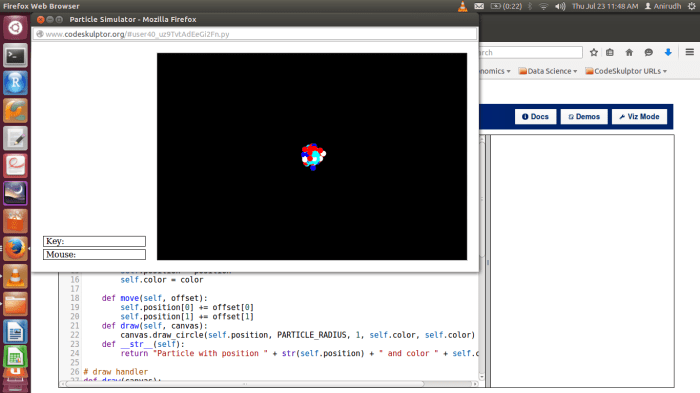
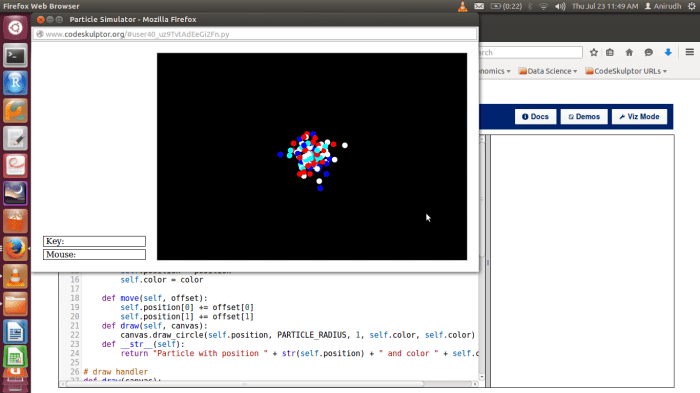
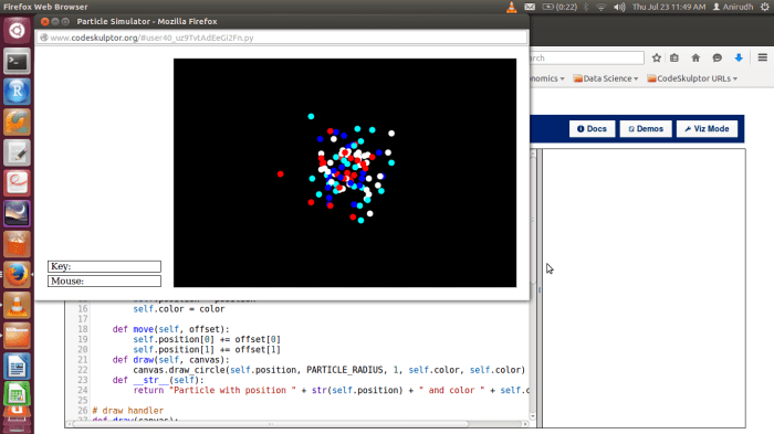
With the help of Rice University’s awesome classes on Python programming I created a cool simulation of particles diffusing into space, using the concept of Classes, which I learnt just yesterday!

Click to check out the code !

Screenshot from 2015-07-23 11:49:00

Screenshot from 2015-07-23 11:49:10

Screenshot from 2015-07-23 11:49:39

Statistics: The Sexiest Job of the Decade

Anyone who’s got a formal education in economics knows who Hal Varian is. He’s most popularly known for his book Intermediate Economics. He’s also the Chief Economist at Google. He is known to have famously stated more or less, that statisticians and data analysts would be the sexiest jobs of the next decade.

That has come true, to a great extent, and we’ll be seeing more.

Great places to learn more about data science and statistical learning:
1] Statistical Learning (Stanford)
2] The Analytics Edge (MIT)

In a paper called ‘Big Data: New Tricks for Econometrics‘, Varian goes on to say that:

In fact, my standard advice to graduate students these days is “go to the computer science department and take a class in machine learning.” There have been very fruitful collaborations between computer scientists and statisticians in the last decade or so, and I expect collaborations between computer scientists and econometricians will also be productive in the future.

See Also: Slides on Machine Learning and Econometrics

Algorithmic Game Theory Lecture Videos and Notes

Link to Stanford professor, Tim Roughgarden’s video lectures on algorithmic game theory (AGT):

2013 Iteration
http://theory.stanford.edu/~tim/f13/f13.html

2014 Iteration
http://theory.stanford.edu/~tim/f14/f14.html

I’m currently doing his Coursera MOOC on algorithms, divided into 2 parts:

https://www.coursera.org/course/algo
https://www.coursera.org/course/algo2

Turing's Invisible Hand

I’m teaching my algorithmic game theory course at Stanford this quarter, and this time around I’m posting lecture videos and notes.  The videos are a static shot of my blackboard lectures, not MOOC-style videos.

The course home page is here.  Week 1 videos and notes, covering several motivating examples and some mechanism design basics, are already available.  This week (Week 2) we’ll prove the correspondence between monotone and implementable allocation rules in single-parameter environments, and introduce algorithmic mechanism design via Knapsack auctions.

The ten-week course has roughly four weeks of lectures on mechanism design, three weeks on the inefficiency of equilibria (e.g., the price of anarchy), and three weeks on algorithms for and the complexity of learning and computing equilibria. Periodically, I’ll post updates on the course content in this space.  I would be very happy to receive comments, corrections, and criticisms on the course organization and content.

View original post

Visualizing Macroeconomic Data using Choropleths in R

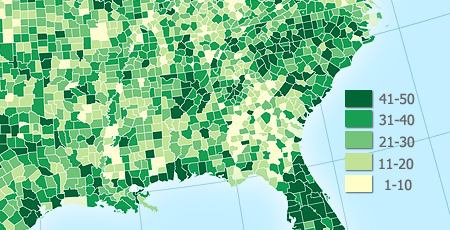
Choropleths are thematic maps shaded or patterned in proportion to the measurement of the statistical variable being displayed on the map, such as population density or per-capita-income.

example choropleth

This post is about creating quick choropleth maps in R, with macroeconomic data across geographies.

As a sample exercise, I decided to get data on what percentage of their aggregate disbursements, do states in India spend on development expenditure. I got the data from the Reserve Bank of India’s website. I had to clean the data a little for easy handling in R. Here’s the cleaned data.

I used the choroplethr package designed by Ari Lamstein and Brian P Johnson to animate the data on the map of India. Here’s my code followed by output maps.

## load the requisite libraries into R
library("xlsx")
library("choroplethr")
library("choroplethrAdmin1")
library("ggplot2")
indianregions <- get_admin1_regions("india")
## gets dataframe of 2 columns with name of country ("india") throughout column 1
## and name of regions in 2nd column
nrow(indianregions)
## counts the number of regions under country "india"
setwd("C:/Anirudh/Coding/R/Practice/Practice Iteration 2")
df_dev_indicators <- read.xlsx("statewise_development_indicators.xls", sheetIndex = 1, colIndex = 2:5, rowIndex = 2:31, header = FALSE)
## reads excel data into an R dataframe
df_dev_indicators_2012 <- df_dev_indicators[c(1,2)]
df_dev_indicators_2013 <- df_dev_indicators[c(1,3)]
df_dev_indicators_2014 <- df_dev_indicators[c(1,4)]
## create 3 separate dataframes from the parent dataframe so as to have 2 columns,
## column 1 for region and column 2 for column 2 for value metric
names(df_dev_indicators_2012) <- c("region","value")
names(df_dev_indicators_2013) <- c("region","value")
names(df_dev_indicators_2014) <- c("region","value")
## assigning column names [required as per choroplethr function]
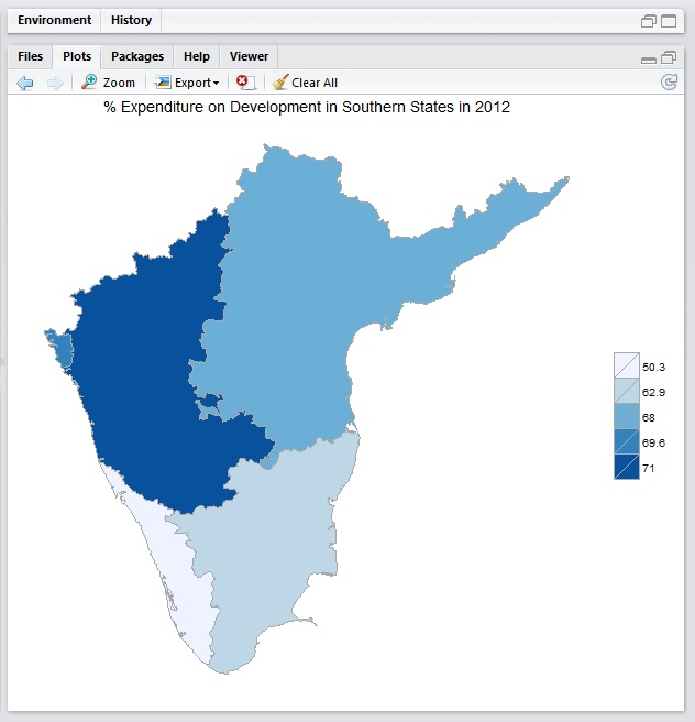
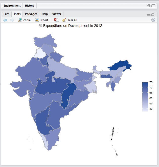
admin1_choropleth("india", df_dev_indicators_2012, title = "% Expenditure on Development in 2012", legend = "", buckets = 9, zoom = NULL)
## prints the choropleth map for 2012 indicators
southern_states <- c("state of karnataka","state of andhra pradesh", "state of kerala", "state of tamil nadu", "state of goa")
## stores regions that are to be printed as a bucket map
admin1_choropleth("india", df_dev_indicators_2012, title = "% Expenditure on Development in Southern States in 2012", legend = "", buckets = 9, zoom = southern_states)
## zooms into the buckets specified earlier
## --- CONTINUOUS SCALE ---
admin1_choropleth("india", df_dev_indicators_2012, title = "% Expenditure on Development in 2012", legend = "", buckets = 1, zoom = NULL)
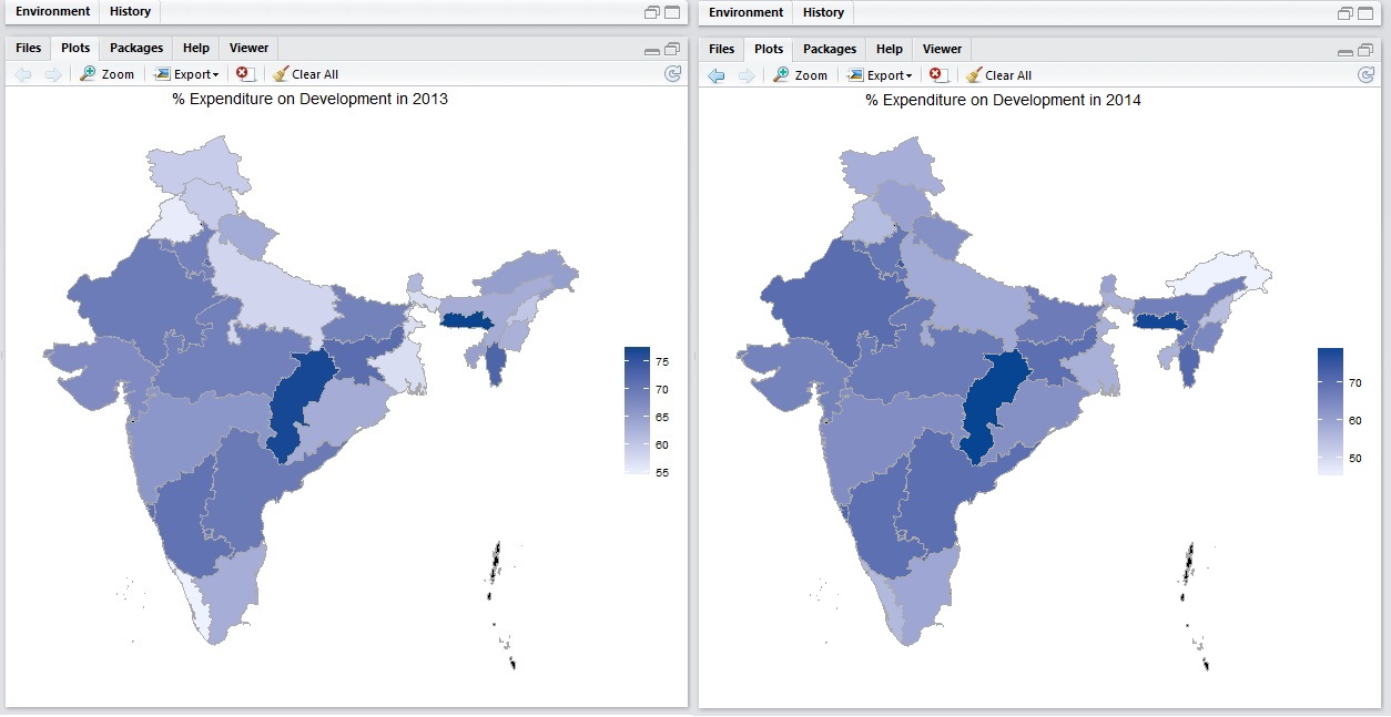
admin1_choropleth("india", df_dev_indicators_2013, title = "% Expenditure on Development in 2013", legend = "", buckets = 1, zoom = NULL)
admin1_choropleth("india", df_dev_indicators_2014, title = "% Expenditure on Development in 2014", legend = "", buckets = 1, zoom = NULL)
view raw choroplethr.R hosted with ❤ by GitHub

…and as expected, the lines of code above print out the desired map

Expenditure on Development in Southern States (2012)

In the examples above I set the buckets attribute equal to 9. That set the data in discrete scales. Had I set buckets = 1 instead, we would have got a continuous scale of data.

Expenditure on Development (2012)_continuous

The same for the last 2 fiscal years:

Development Expenditures in the Last 2 Years

For the US, there are amazing packages for county level and ZIP code level detail of data visualization.

Here’s more on the choroplethr package for R and creating your own maps.

Hello World!

Hello World

Hi all!

This website would be a most unusual way to blog about programming languages, that too coming from someone who hasn’t done much coding. In the next few minutes, I offer an introduction. It’s divided into 2 parts.

(i) introducing myself
(ii) an introduction to WHY I created this blog

Intro (i)

I am an electrical engineer who took to finance after graduating from college — doing what I’d like to think was preparing client pitches that bankers would use to wrap up multi-million dollar deals!

Just kidding. All I was doing was waiting for the last day of the month for the salary figure to pop up as a message in my phone’s inbox, i.e., watching my bank balance go up every month. It was in a moment of epiphany that I realized that I had better quit before I got used to being that way.

I then spent some time working as a social media analyst for a revolutionary political outfit — around the same time when the capital city of India was going to the polls for the Assembly elections. Politics sparked my curiosity for what was coming next – Economics!

I fell in love immediately, which found me studying economics here, at a research institute funded by the RBI, India’s equivalent of the Fed. I braved a semester, managing a face-saving GPA, for it had been 3 years since I had left academics, and I was moving to something unrelated to what I had been doing in the past, so the transition couldn’t have been smooth, I knew that.

Nevertheless, when I was taking my end of term exams that semester, it was after 2 weeks of hitting the gym. But life has its ways of throwing lemons at us from time to time. I’m now trying to squeeze the juice out of them for the proverbial lemonade. Anyway, I had to cut short my attempts at acquiring a six pack when it started to pain in my pelvic region, and my right leg had gone numb. Through the pain I somehow managed to appear for the end terms. When I was home after my exams, the pain gradually got worse and rose — like a crescendo!

Intro (ii)

Turns out I had what is commonly known as a slipped disc. I had herniations in L4-L5 and L5-S1 discs of my spine, with a 100% prolapse in the latter.

It’s been very painful. I can’t sit for more than 5 minutes without getting muscular spasms in my lumbar region, numbness in my feet and distressing nerve pain in my toes, buttocks and thighs that last for a couple of days each time I try sitting. Can’t stand longer than 10 minutes.

In summary, I’ve been bedridden for over 16 weeks now and have 9 months ahead of me before I can continue my education from where I had to leave it. Staying confined in a room for months on end, sick, is worse than being locked up in prison. It makes going to the doctor seem like a picnic!

I always wanted to get my hands dirty with programming, so I decided after much deliberation, that I would learn as much of Python and R as I can in the coming months. I’ll talk more about WHY, in some of my future posts (like this one), but for now it should suffice if I told you I want to keep myself from getting bored to death. For the months of April through December, this blog is meant to document my learning and struggles, insights and revelations.

What better way to start than this —

> print(“Hello World”)  # R
>>> print “Hello World”  # Python