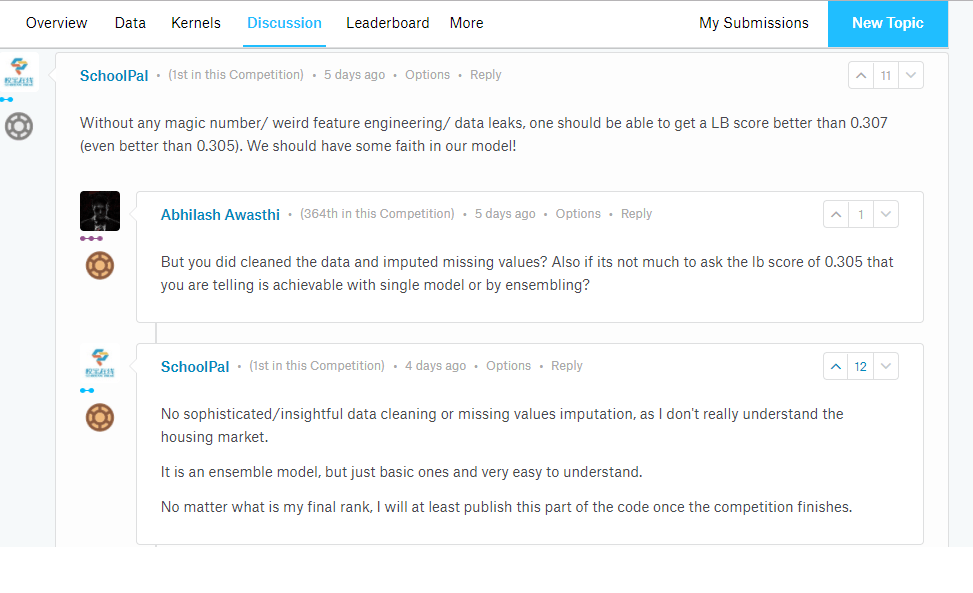
I’ve been stuck for about a week at the 52nd percentile among 3400+ Kagglers taking part in the competition. I’ve been told that Kaggle Kernels and discussion boards are helpful when you’re stuck or if you need to learn some practical data science that can’t be gleaned from books or tutorials.
One such discussion thread looks like this:
This person going by the pseudonym Schoolpal is currently killing it on the leaderboard and I’m eagerly looking forward to this person’s code once the competition ends in less than 24 hours. If you’re interested too, follow this discussion here.
Cheers!
Update:
This Schoolpal, as mentioned earlier, finally came in second and shared their approach here.
This was in the pipeline for quite some time now. I have been waiting for his lectures on a platform such as EdX or Coursera, and the day has arrived. You can enroll and start with week 1’s lectures as they’re live now.
This course is taught by none other than Dr. Yaser S. Abu – Mostafa, whose textbook on machine learning, Learning from Data is #1 bestseller textbook (Amazon) in all categories of Computer Science. His online course has been offered earlier over here.
Teaching
Dr. Abu-Mostafa received the Clauser Prize for the most original doctoral thesis at Caltech. He received the ASCIT Teaching Awards in 1986, 1989 and 1991, the GSC Teaching Awards in 1995 and 2002, and the Richard P. Feynman prize for excellence in teaching in 1996.
Live ‘One-take’ Recordings
The lectures have been recorded from a live broadcast (including Q&A, which will let you gauge the level of CalTech students taking this course). In fact, it almost seems as though Abu Mostafa takes a direct jab at Andrew Ng’s popular Coursera MOOC by stating the obvious on his course page.
A real Caltech course, not a watered-down version
Again, while enrolling note that this is what Abu Mostafa had to say about the online course: “A Caltech course does not cater to short attention spans, and it may not provide instant gratification…[like] many MOOCs out there that are quite simple and have a ‘video game’ feel to them.” Unsurprisingly, many online students have dropped out in the past, but some of those students who “complained early on but decided to stick with the course had very flattering words to say at the end”.
Prerequisites
Basic probability
Basic matrices
Basic calculus
Some programming language/platform (I choose Python!)
If you’re looking for a challenging machine learning course, this is probably one you must take.
Disclaimer: I’m not a data scientist yet. That’s still work in progress, but I’d recommend this excellent talk given by Tetiana Ivanova to put an enthusiast’s data science journey in perspective.
This happens to be my 50th blog post – and my blog is 8 months old.
🙂
This post is the third and last post in in a series of posts (Part 1 – Part 2) on data manipulation with dlpyr. Note that the objects in the code may have been defined in earlier posts and the code in this post is in continuation with code from the earlier posts.
Although datasets can be manipulated in sophisticated ways by linking the 5 verbs of dplyr in conjunction, linking verbs together can be a bit verbose.
Creating multiple objects, especially when working on a large dataset can slow you down in your analysis. Chaining functions directly together into one line of code is difficult to read. This is sometimes called the Dagwood sandwich problem: you have too much filling (too many long arguments) between your slices of bread (parentheses). Functions and arguments get further and further apart.
The %>% operator allows you to extract the first argument of a function from the arguments list and put it in front of it, thus solving the Dagwood sandwich problem.
This file contains hidden or bidirectional Unicode text that may be interpreted or compiled differently than what appears below. To review, open the file in an editor that reveals hidden Unicode characters.
Learn more about bidirectional Unicode characters
group_by() defines groups within a data set. Its influence becomes clear when calling summarise() on a grouped dataset. Summarizing statistics are calculated for the different groups separately.
This file contains hidden or bidirectional Unicode text that may be interpreted or compiled differently than what appears below. To review, open the file in an editor that reveals hidden Unicode characters.
Learn more about bidirectional Unicode characters
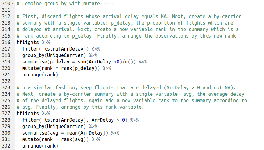
group_by() can also be combined with mutate(). When you mutate grouped data, mutate() will calculate the new variables independently for each group. This is particularly useful when mutate() uses the rank() function, that calculates within group rankings. rank() takes a group of values and calculates the rank of each value within the group, e.g.
rank(c(21, 22, 24, 23))
has output
[1] 1 2 4 3
As with arrange(), rank() ranks values from the largest to the smallest and this behaviour can be reversed with the desc() function.
This file contains hidden or bidirectional Unicode text that may be interpreted or compiled differently than what appears below. To review, open the file in an editor that reveals hidden Unicode characters.
Learn more about bidirectional Unicode characters
So after 8 months of playing around with R and Python and blog post after blog post, I found myself finally hacking away at a problem set from the 17th storey of the Hindustan Times building at Connaught Place. I had entered my first ever data science hackathon conducted by Analytics Vidhya, a pioneer in analytics learning in India. Pizzas and Pepsi were on the house. Like any predictive analysis hackathon, this one accepted unlimited entries till submission time. It was from 2pm to 4:30pm today – 2.5 hours, of which I ended up wasting 1.5 hours trying to make my first submission which encountered submission error after submission error until the problem was fixed finally post lunch. I had 1 hour to try my best. It wasn’t the best performance, but I thought of blogging this experience anyway, as a reminder of the work that awaits me. I want to be the one winning prize money at the end of the day.
Note that this post is in continuation with Part 1 of this series of posts on data manipulation with dplyr in R. The code in this post carries forward from the variables / objects defined in Part 1.
In the previous post, I talked about how dplyr provides a grammar of sorts to manipulate data, and consists of 5 verbs to do so:
The 5 verbs of dplyr select – removes columns from a dataset filter – removes rows from a dataset arrange – reorders rows in a dataset mutate – uses the data to build new columns and values summarize – calculates summary statistics
I went on to discuss examples using select() and mutate(). Let’s now talk about filter(). R comes with a set of logical operators that you can use inside filter(). These operators are: x < y,TRUE if x is less than y x <= y, TRUE if x is less than or equal to y x == y, TRUE if x equals y x != y, TRUE if x does not equal y x >= y, TRUE if x is greater than or equal to y x > y, TRUE if x is greater than y x %in% c(a, b, c), TRUE if x is in the vector c(a, b, c)
The following call, for example, filters df such that only the observations where the variable a is greater than the variable b: filter(df, a > b)
This file contains hidden or bidirectional Unicode text that may be interpreted or compiled differently than what appears below. To review, open the file in an editor that reveals hidden Unicode characters.
Learn more about bidirectional Unicode characters
Combining tests using boolean operators
R also comes with a set of boolean operators that you can use to combine multiple logical tests into a single test. These include & (and), | (or), and ! (not). Instead of using the & operator, you can also pass several logical tests to filter(), separated by commas. The following calls equivalent:
filter(df, a > b & c > d) filter(df, a > b, c > d)
The is.na() will also come in handy very often. This expression, for example, keeps the observations in df for which the variable x is not NA:
filter(df, !is.na(x))
This file contains hidden or bidirectional Unicode text that may be interpreted or compiled differently than what appears below. To review, open the file in an editor that reveals hidden Unicode characters.
Learn more about bidirectional Unicode characters
This file contains hidden or bidirectional Unicode text that may be interpreted or compiled differently than what appears below. To review, open the file in an editor that reveals hidden Unicode characters.
Learn more about bidirectional Unicode characters
Arranging Data arrange() can be used to rearrange rows according to any type of data. If you pass arrange() a character variable, R will rearrange the rows in alphabetical order according to values of the variable. If you pass a factor variable, R will rearrange the rows according to the order of the levels in your factor (running levels() on the variable reveals this order).
By default, arrange() arranges the rows from smallest to largest. Rows with the smallest value of the variable will appear at the top of the data set. You can reverse this behaviour with the desc() function. arrange() will reorder the rows from largest to smallest values of a variable if you wrap the variable name in desc() before passing it to arrange()
This file contains hidden or bidirectional Unicode text that may be interpreted or compiled differently than what appears below. To review, open the file in an editor that reveals hidden Unicode characters.
Learn more about bidirectional Unicode characters
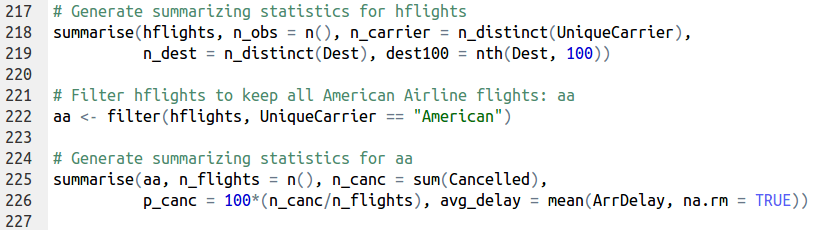
summarise(), the last of the 5 verbs, follows the same syntax as mutate(), but the resulting dataset consists of a single row instead of an entire new column in the case of mutate().
In contrast to the four other data manipulation functions, summarise() does not return an altered copy of the dataset it is summarizing; instead, it builds a new dataset that contains only the summarizing statistics.
Note:summarise() and summarize() both work the same!
You can use any function you like in summarise(), so long as the function can take a vector of data and return a single number. R contains many aggregating functions. Here are some of the most useful:
min(x) – minimum value of vector x. max(x) – maximum value of vector x. mean(x) – mean value of vector x. median(x) – median value of vector x. quantile(x, p) – pth quantile of vector x. sd(x) – standard deviation of vector x. var(x) – variance of vector x. IQR(x) – Inter Quartile Range (IQR) of vector x. diff(range(x)) – total range of vector x.
This file contains hidden or bidirectional Unicode text that may be interpreted or compiled differently than what appears below. To review, open the file in an editor that reveals hidden Unicode characters.
Learn more about bidirectional Unicode characters
dplyr provides several helpful aggregate functions of its own, in addition to the ones that are already defined in R. These include:
first(x) – The first element of vector x. last(x) – The last element of vector x. nth(x, n) – The nth element of vector x. n() – The number of rows in the data.frame or group of observations that summarise() describes. n_distinct(x) – The number of unique values in vector x
This file contains hidden or bidirectional Unicode text that may be interpreted or compiled differently than what appears below. To review, open the file in an editor that reveals hidden Unicode characters.
Learn more about bidirectional Unicode characters
This would be it for Part-2 of this series of posts on data manipulation with dplyr. Part 3 would focus on the pipe operator, Group_by and working with databases.
dplyr is one of the packages in R that makes R so loved by data scientists. It has three main goals:
Identify the most important data manipulation tools needed for data analysis and make them easy to use in R.
Provide blazing fast performance for in-memory data by writing key pieces of code in C++.
Use the same code interface to work with data no matter where it’s stored, whether in a data frame, a data table or database.
Introduction to the dplyr package and the tbl class
This post is mostly about code. If you’re interested in learning dplyr I recommend you type in the commands line by line on the R console to see first hand what’s happening.
This file contains hidden or bidirectional Unicode text that may be interpreted or compiled differently than what appears below. To review, open the file in an editor that reveals hidden Unicode characters.
Learn more about bidirectional Unicode characters
Select and mutate dplyr provides grammar for data manipulation apart from providing data structure. The grammar is built around 5 functions (also referred to as verbs) that do the basic tasks of data manipulation.
The 5 verbs of dplyr select – removes columns from a dataset filter – removes rows from a dataset arrange – reorders rows in a dataset mutate – uses the data to build new columns and values summarize – calculates summary statistics
dplyr functions do not change the dataset. They return a new copy of the dataset to use.
To answer the simple question whether flight delays tend to shrink or grow during a flight, we can safely discard a lot of the variables of each flight. To select only the ones that matter, we can use select()
This file contains hidden or bidirectional Unicode text that may be interpreted or compiled differently than what appears below. To review, open the file in an editor that reveals hidden Unicode characters.
Learn more about bidirectional Unicode characters
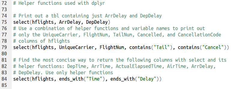
dplyr comes with a set of helper functions that can help you select variables. These functions find groups of variables to select, based on their names. Each of these works only when used inside of select()
starts_with(“X”): every name that starts with “X”
ends_with(“X”): every name that ends with “X”
contains(“X”): every name that contains “X”
matches(“X”): every name that matches “X”, where “X” can be a regular expression
num_range(“x”, 1:5): the variables named x01, x02, x03, x04 and x05
one_of(x): every name that appears in x, which should be a character vector
This file contains hidden or bidirectional Unicode text that may be interpreted or compiled differently than what appears below. To review, open the file in an editor that reveals hidden Unicode characters.
Learn more about bidirectional Unicode characters
In order to appreciate the usefulness of dplyr, here are some comparisons between base R and dplyr
This file contains hidden or bidirectional Unicode text that may be interpreted or compiled differently than what appears below. To review, open the file in an editor that reveals hidden Unicode characters.
Learn more about bidirectional Unicode characters
mutate() is the second of the five data manipulation functions. mutate() creates new columns which are added to a copy of the dataset.
This file contains hidden or bidirectional Unicode text that may be interpreted or compiled differently than what appears below. To review, open the file in an editor that reveals hidden Unicode characters.
Learn more about bidirectional Unicode characters
So far we have added variables to hflights one at a time, but we can also use mutate() to add multiple variables at once.
This file contains hidden or bidirectional Unicode text that may be interpreted or compiled differently than what appears below. To review, open the file in an editor that reveals hidden Unicode characters.
Learn more about bidirectional Unicode characters
Although the lecture videos and lecture notes from Andrew Ng‘s Coursera MOOC are sufficient for the online version of the course, if you’re interested in more mathematical stuff or want to be challenged further, you can go through the following notes and problem sets from CS 229, a 10-week course that he teaches at Stanford (which also happens to be the most enrolled course on campus). It’s not hard to end up with a 100% score on his MOOC which is obviously a (much) watered down version of the course he teaches at Stanford, at least in terms of difficulty. If you don’t believe me, just have a go at the problem sets from the links below.
MIT’s Fall 2015 iteration of 6.00.2xstarts today. After an enriching learning experience with 6.00.1x, I have great expectations from this course. As the course website mildly puts it, 6.00.2x is an introduction to using computation to understand real-world phenomena. MIT OpenCourseware (OCW) mirroring the material covered in 6.00.1x and 6.00.2x can be found here.
The course follows this book by John Guttag (who happens to be one of the instructors for this course). However, purchasing the book isn’t a necessity for this course.
One thing I loved about 6.00.1x was its dedicated Facebook group, which gave a community / classroom-peergroup feel to the course. 6.00.2x also has a Facebook group. Here’s a sneak peak:
Thesyllabus and schedule for this course is shown below. The course is spread out over 2 months which includes 7 weeks of lectures.
MITx 6.00.2x Fall 2015 Course Calendar
The prerequisites for this course are pretty much covered in this set of tutorial videos that have been created by one of the TAs for 6.00.1x. If you’ve not taken 6.00.1x in the past, you can go through these videos (running time < 1hr) to judge whether or not to go ahead with 6.00.2x.
It has been 3 years since I have steered my interests towards Machine Learning. I had just graduated from college with a Bachelor of Engineering in Electronics and Communication Engineering. Which is, other way of saying that I was:
a toddler in programming.
little / no knowledge of algorithms.
studied engineering math, but it was rusty.
no knowledge of modern optimization.
zero knowledge of statistical inference.
I think, most of it is true for many engineering graduates (especially, in India !). Unless, you studied mathematics and computing for undergrad.
Lucky for me, I had a great mentor and lot of online materials on these topics. This post will list many such materials I found useful, while I was learning it the hard way !
All the courses that I’m listing below have homework assignments. Make sure you work through each one of them.