Spot the Difference — It’s NumPy!

My first brush with NumPy happened over writing a block of code to make a plot using pylab. ⇣


pylab is part of matplotlib (in matplotlib.pylab) and tries to give you a MatLab like environment. matplotlib has a number of dependencies, among them numpy which it imports under the common alias np. scipy is not a dependency of matplotlib.


I had a tuple (of lows and highs of temperature) of lengh 2 with 31 entries in each (the number of days in the month of July), parsed from this text file:

Boston July Temperatures
-------------------------
Day High Low
------------
1 91 70
2 84 69
3 86 68
4 84 68
5 83 70
6 80 68
7 86 73
8 89 71
9 84 67
10 83 65
11 80 66
12 86 63
13 90 69
14 91 72
15 91 72
16 88 72
17 97 76
18 89 70
19 74 66
20 71 64
21 74 61
22 84 61
23 86 66
24 91 68
25 83 65
26 84 66
27 79 64
28 72 63
29 73 64
30 81 63
31 73 63
view raw julyTemps.txt hosted with ❤ by GitHub

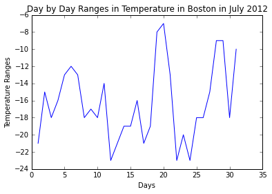
Given below, are 2 sets of code that do the same thing; one without NumPy and the other with NumPy. They output the following graph using PyLab:

differenceTemp

Code without NumPy

import pylab
def loadfile():
inFile = open('julyTemps.txt', 'r')
high =[]; low = []
for line in inFile:
fields = line.split()
if len(fields) < 3 or not fields[0].isdigit():
pass
else:
high.append(int(fields[1]))
low.append(int(fields[2]))
return low, high
def producePlot(lowTemps, highTemps):
diffTemps = [highTemps[i] - lowTemps[i] for i in range(len(lowTemps))]
pylab.title('Day by Day Ranges in Temperature in Boston in July 2012')
pylab.xlabel('Days')
pylab.ylabel('Temperature Ranges')
return pylab.plot(range(1,32),diffTemps)
producePlot(loadfile()[1], loadfile()[0])
view raw withoutNumPy.py hosted with ❤ by GitHub

Code with NumPy
import pylab
import numpy as np
def loadFile():
inFile = open('julyTemps.txt')
high = [];vlow = []
for line in inFile:
fields = line.split()
if len(fields) != 3 or 'Boston' == fields[0] or 'Day' == fields[0]:
continue
else:
high.append(int(fields[1]))
low.append(int(fields[2]))
return (low, high)
def producePlot(lowTemps, highTemps):
diffTemps = list(np.array(highTemps) - np.array(lowTemps))
pylab.plot(range(1,32), diffTemps)
pylab.title('Day by Day Ranges in Temperature in Boston in July 2012')
pylab.xlabel('Days')
pylab.ylabel('Temperature Ranges')
pylab.show()
(low, high) = loadFile()
producePlot(low, high)
view raw withNumPy.py hosted with ❤ by GitHub

The difference in code lies in how the variable diffTemps is calculated.

diffTemps = list(np.array(highTemps) - np.array(lowTemps))

seems more readable than

diffTemps = [highTemps[i] - lowTemps[i] for i in range(len(lowTemps))]

Notice how straight forward it is with NumPy. At the core of the NumPy package, is the ndarray object. This encapsulates n-dimensional arrays of homogeneous data types, with many operations being performed in compiled code for performance. element-by-element operations are the “default mode” when an ndarray is involved, but the element-by-element operation is speedily executed by pre-compiled C code.

Advertisement

MITx 6.00.2x Introduction to Computational Thinking and Data Science (Fall 2015)

MIT’s Fall 2015 iteration of 6.00.2x starts today. After an enriching learning experience with 6.00.1x, I have great expectations from this course. As the course website mildly puts it, 6.00.2x is an introduction to using computation to understand real-world phenomena. MIT OpenCourseware (OCW) mirroring the material covered in 6.00.1x and 6.00.2x can be found here.

The course follows this book by John Guttag (who happens to be one of the instructors for this course). However, purchasing the book isn’t a necessity for this course.

Introduction to Computation and Programming Using Python

One thing I loved about 6.00.1x was its dedicated Facebook group, which gave a community / classroom-peergroup feel to the course. 6.00.2x also has a Facebook group. Here’s a sneak peak:

descriptionUpdate

The syllabus and schedule for this course is shown below. The course is spread out over 2 months which includes 7 weeks of lectures.

MITx 6.00.2x Fall 2015 Course Calendar

The prerequisites for this course are pretty much covered in this set of tutorial videos that have been created by one of the TAs for 6.00.1x. If you’ve not taken 6.00.1x in the past, you can go through these videos (running time < 1hr) to judge whether or not to go ahead with 6.00.2x.

So much for the update. Got work to do! 🙂

Object Oriented Programing with Python – Particle Diffusion Simulation

I’m a newbie to the programming world. I first started programming in Python in May this year, a month after I started this blog, so I still haven’t learnt enough to contribute to economics as is the stated goal of this blog. But I know I’ll get there in a year or less.

This blog was also meant to document my learning. In May, I would have called myself Newb v0.0. Today, 3 months later, I’d like to call myself Newb v0.3 and the goal is to be at least Expert v1.0 by January 2016.

With the help of Rice University’s awesome classes on Python programming I created a cool simulation of particles diffusing into space, using the concept of Classes, which I learnt just yesterday!

Click to check out the code !

Screenshot from 2015-07-23 11:49:00

Screenshot from 2015-07-23 11:49:10

Screenshot from 2015-07-23 11:49:39

Introducing cricketr! : An R package to analyze performances of cricketers

Wicked! Or must I say ‘howzzat!?’

Giga thoughts ...

Yet all experience is an arch wherethro’
Gleams that untravell’d world whose margin fades
For ever and forever when I move.
How dull it is to pause, to make an end,
To rust unburnish’d, not to shine in use!

Ulysses by Alfred Tennyson

Introduction

This is an initial post in which I introduce a cricketing package ‘cricketr’ which I have created. This package was a natural culmination to my earlier posts on cricket and my completing 9 modules of Data Science Specialization, from John Hopkins University at Coursera. The thought of creating this package struck me some time back, and I have finally been able to bring this to fruition.

So here it is. My R package ‘cricketr!!!’

This package uses the statistics info available in ESPN Cricinfo Statsguru. The current version of this package only uses data from test cricket. I plan to develop functionality for One-day and…

View original post 4,951 more words

One-Month-Old Blog

UPDATE: While I’m already half way through the much recommended book by Zed A. Shaw – Learn Python The Hard Way, I’m still doing my research on other great resources to help me get started with Python. This page listing 10 Python blogs worth following, in particular emphasizes Mouse vs python to be the most useful. Starting the 10th of June, I’ll be engaged on a 9-week-long MOOC on Computer Science using Python, offered by MIT.

It’s been 2 months since I got started with R, and although my progress seems fast to me, it appears so mainly because R comes with insanely helpful packages that reduce large chunks of code into simple functions. Not only that, data visualization and graphics generated in R are beautiful and elegant. For example, the following code generates a Mandelbrot set created through the first 50 iterations of equation z = z2 + c plotted for different complex constants c

library(caTools)         # external package providing write.gif function
jet.colors <- colorRampPalette(c("#00007F", "blue", "#007FFF", "cyan", "#7FFF7F",
                                 "yellow", "#FF7F00", "red", "#7F0000"))
m <- 1000                # define size
C <- complex( real=rep(seq(-1.8,0.6, length.out=m), each=m ),
              imag=rep(seq(-1.2,1.2, length.out=m), m ) )
C <- matrix(C,m,m)       # reshape as square matrix of complex numbers
Z <- 0                   # initialize Z to zero
X <- array(0, c(m,m,50)) # initialize output 3D array
for (k in 1:50) {        # loop with 50 iterations
  Z <- Z^2+C             # the central difference equation
  X[,,k] <- exp(-abs(Z)) # capture results
}
write.gif(X, "Mandelbrot.gif", col=jet.colors, delay=800)

Mandelbrot

This is just an illustration of the power of a dozen or so lines of R code. Just as there are a ridiculous many packages in R, there are countless modules packed into many thousands of packages in Python to make life simpler, so I wasn’t surprised to find a module called antigravity, that can be imported in Python like this:

 import antigravity  

and voila, you are redirected to this telling XKCD tale of Cueball performing gravity-defying stunts with Python.

source: http://www.xkcd.com/353/

Visualizing Macroeconomic Data using Choropleths in R

Choropleths are thematic maps shaded or patterned in proportion to the measurement of the statistical variable being displayed on the map, such as population density or per-capita-income.

example choropleth

This post is about creating quick choropleth maps in R, with macroeconomic data across geographies.

As a sample exercise, I decided to get data on what percentage of their aggregate disbursements, do states in India spend on development expenditure. I got the data from the Reserve Bank of India’s website. I had to clean the data a little for easy handling in R. Here’s the cleaned data.

I used the choroplethr package designed by Ari Lamstein and Brian P Johnson to animate the data on the map of India. Here’s my code followed by output maps.

## load the requisite libraries into R
library("xlsx")
library("choroplethr")
library("choroplethrAdmin1")
library("ggplot2")
indianregions <- get_admin1_regions("india")
## gets dataframe of 2 columns with name of country ("india") throughout column 1
## and name of regions in 2nd column
nrow(indianregions)
## counts the number of regions under country "india"
setwd("C:/Anirudh/Coding/R/Practice/Practice Iteration 2")
df_dev_indicators <- read.xlsx("statewise_development_indicators.xls", sheetIndex = 1, colIndex = 2:5, rowIndex = 2:31, header = FALSE)
## reads excel data into an R dataframe
df_dev_indicators_2012 <- df_dev_indicators[c(1,2)]
df_dev_indicators_2013 <- df_dev_indicators[c(1,3)]
df_dev_indicators_2014 <- df_dev_indicators[c(1,4)]
## create 3 separate dataframes from the parent dataframe so as to have 2 columns,
## column 1 for region and column 2 for column 2 for value metric
names(df_dev_indicators_2012) <- c("region","value")
names(df_dev_indicators_2013) <- c("region","value")
names(df_dev_indicators_2014) <- c("region","value")
## assigning column names [required as per choroplethr function]
admin1_choropleth("india", df_dev_indicators_2012, title = "% Expenditure on Development in 2012", legend = "", buckets = 9, zoom = NULL)
## prints the choropleth map for 2012 indicators
southern_states <- c("state of karnataka","state of andhra pradesh", "state of kerala", "state of tamil nadu", "state of goa")
## stores regions that are to be printed as a bucket map
admin1_choropleth("india", df_dev_indicators_2012, title = "% Expenditure on Development in Southern States in 2012", legend = "", buckets = 9, zoom = southern_states)
## zooms into the buckets specified earlier
## --- CONTINUOUS SCALE ---
admin1_choropleth("india", df_dev_indicators_2012, title = "% Expenditure on Development in 2012", legend = "", buckets = 1, zoom = NULL)
admin1_choropleth("india", df_dev_indicators_2013, title = "% Expenditure on Development in 2013", legend = "", buckets = 1, zoom = NULL)
admin1_choropleth("india", df_dev_indicators_2014, title = "% Expenditure on Development in 2014", legend = "", buckets = 1, zoom = NULL)
view raw choroplethr.R hosted with ❤ by GitHub

…and as expected, the lines of code above print out the desired map

Expenditure on Development in Southern States (2012)

In the examples above I set the buckets attribute equal to 9. That set the data in discrete scales. Had I set buckets = 1 instead, we would have got a continuous scale of data.

Expenditure on Development (2012)_continuous

The same for the last 2 fiscal years:

Development Expenditures in the Last 2 Years

For the US, there are amazing packages for county level and ZIP code level detail of data visualization.

Here’s more on the choroplethr package for R and creating your own maps.