My first brush with NumPy happened over writing a block of code to make a plot using pylab. ⇣
pylabis part ofmatplotlib(inmatplotlib.pylab) and tries to give you a MatLab like environment.matplotlibhas a number of dependencies, among themnumpywhich it imports under the common aliasnp.scipyis not a dependency ofmatplotlib.
I had a tuple (of lows and highs of temperature) of lengh 2 with 31 entries in each (the number of days in the month of July), parsed from this text file:
| Boston July Temperatures | |
| ————————- | |
| Day High Low | |
| ———— | |
| 1 91 70 | |
| 2 84 69 | |
| 3 86 68 | |
| 4 84 68 | |
| 5 83 70 | |
| 6 80 68 | |
| 7 86 73 | |
| 8 89 71 | |
| 9 84 67 | |
| 10 83 65 | |
| 11 80 66 | |
| 12 86 63 | |
| 13 90 69 | |
| 14 91 72 | |
| 15 91 72 | |
| 16 88 72 | |
| 17 97 76 | |
| 18 89 70 | |
| 19 74 66 | |
| 20 71 64 | |
| 21 74 61 | |
| 22 84 61 | |
| 23 86 66 | |
| 24 91 68 | |
| 25 83 65 | |
| 26 84 66 | |
| 27 79 64 | |
| 28 72 63 | |
| 29 73 64 | |
| 30 81 63 | |
| 31 73 63 |
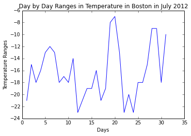
Given below, are 2 sets of code that do the same thing; one without NumPy and the other with NumPy. They output the following graph using PyLab:
Code without NumPy
| import pylab | |
| def loadfile(): | |
| inFile = open('julyTemps.txt', 'r') | |
| high =[]; low = [] | |
| for line in inFile: | |
| fields = line.split() | |
| if len(fields) < 3 or not fields[0].isdigit(): | |
| pass | |
| else: | |
| high.append(int(fields[1])) | |
| low.append(int(fields[2])) | |
| return low, high | |
| def producePlot(lowTemps, highTemps): | |
| diffTemps = [highTemps[i] – lowTemps[i] for i in range(len(lowTemps))] | |
| pylab.title('Day by Day Ranges in Temperature in Boston in July 2012') | |
| pylab.xlabel('Days') | |
| pylab.ylabel('Temperature Ranges') | |
| return pylab.plot(range(1,32),diffTemps) | |
| producePlot(loadfile()[1], loadfile()[0]) |
Code with NumPy
| import pylab | |
| import numpy as np | |
| def loadFile(): | |
| inFile = open('julyTemps.txt') | |
| high = [];vlow = [] | |
| for line in inFile: | |
| fields = line.split() | |
| if len(fields) != 3 or 'Boston' == fields[0] or 'Day' == fields[0]: | |
| continue | |
| else: | |
| high.append(int(fields[1])) | |
| low.append(int(fields[2])) | |
| return (low, high) | |
| def producePlot(lowTemps, highTemps): | |
| diffTemps = list(np.array(highTemps) – np.array(lowTemps)) | |
| pylab.plot(range(1,32), diffTemps) | |
| pylab.title('Day by Day Ranges in Temperature in Boston in July 2012') | |
| pylab.xlabel('Days') | |
| pylab.ylabel('Temperature Ranges') | |
| pylab.show() | |
| (low, high) = loadFile() | |
| producePlot(low, high) |
The difference in code lies in how the variable diffTemps is calculated.
diffTemps = list(np.array(highTemps) - np.array(lowTemps))
seems more readable than
diffTemps = [highTemps[i] - lowTemps[i] for i in range(len(lowTemps))]
Notice how straight forward it is with NumPy. At the core of the NumPy package, is the ndarray object. This encapsulates n-dimensional arrays of homogeneous data types, with many operations being performed in compiled code for performance. element-by-element operations are the “default mode” when an ndarray is involved, but the element-by-element operation is speedily executed by pre-compiled C code.
 Anirudh Jayaraman