This was in the pipeline for quite some time now. I have been waiting for his lectures on a platform such as EdX or Coursera, and the day has arrived. You can enroll and start with week 1’s lectures as they’re live now.
This course is taught by none other than Dr. Yaser S. Abu – Mostafa, whose textbook on machine learning, Learning from Data is #1 bestseller textbook (Amazon) in all categories of Computer Science. His online course has been offered earlier over here.
Teaching
Dr. Abu-Mostafa received the Clauser Prize for the most original doctoral thesis at Caltech. He received the ASCIT Teaching Awards in 1986, 1989 and 1991, the GSC Teaching Awards in 1995 and 2002, and the Richard P. Feynman prize for excellence in teaching in 1996.
Live ‘One-take’ Recordings
The lectures have been recorded from a live broadcast (including Q&A, which will let you gauge the level of CalTech students taking this course). In fact, it almost seems as though Abu Mostafa takes a direct jab at Andrew Ng’s popular Coursera MOOC by stating the obvious on his course page.
A real Caltech course, not a watered-down version
Again, while enrolling note that this is what Abu Mostafa had to say about the online course: “A Caltech course does not cater to short attention spans, and it may not provide instant gratification…[like] many MOOCs out there that are quite simple and have a ‘video game’ feel to them.” Unsurprisingly, many online students have dropped out in the past, but some of those students who “complained early on but decided to stick with the course had very flattering words to say at the end”.
Prerequisites
Basic probability
Basic matrices
Basic calculus
Some programming language/platform (I choose Python!)
If you’re looking for a challenging machine learning course, this is probably one you must take.
This file contains hidden or bidirectional Unicode text that may be interpreted or compiled differently than what appears below. To review, open the file in an editor that reveals hidden Unicode characters.
Learn more about bidirectional Unicode characters
This file contains hidden or bidirectional Unicode text that may be interpreted or compiled differently than what appears below. To review, open the file in an editor that reveals hidden Unicode characters.
Learn more about bidirectional Unicode characters
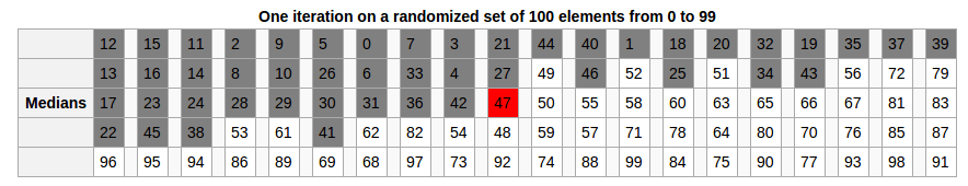
Through this post, I’m sharing Python code implementing the median of medians algorithm, an algorithm that resembles quickselect, differing only in the way in which the pivot is chosen, i.e, deterministically, instead of at random.
Its best case complexity is O(n) and worst case complexity O(nlog2n)
I don’t have a formal education in CS, and came across this algorithm while going through Tim Roughgarden’s Coursera MOOC on the design and analysis of algorithms. Check out my implementation in Python.
This file contains hidden or bidirectional Unicode text that may be interpreted or compiled differently than what appears below. To review, open the file in an editor that reveals hidden Unicode characters.
Learn more about bidirectional Unicode characters
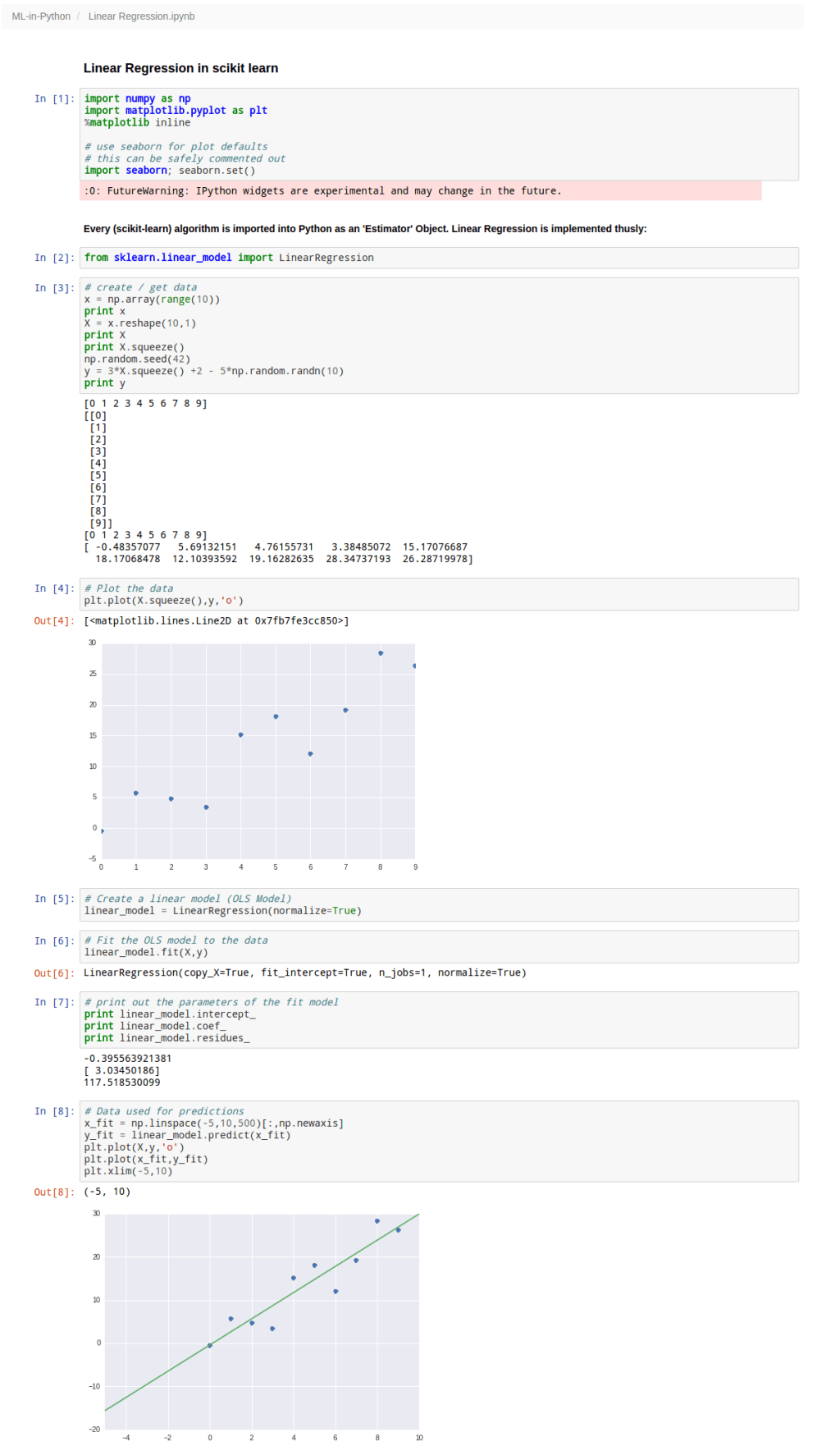
Here’s a quick example case for implementing one of the simplest of learning algorithms in any machine learning toolbox – Linear Regression. You can download the IPython / Jupyter notebook here so as to play around with the code and try things out yourself.
I’m doing a series of posts on scikit-learn. Its documentation is vast, so unless you’re willing to search for a needle in a haystack, you’re better off NOT jumping into the documentation right away. Instead, knowing chunks of code that do the job might help.
Find the kth smallest element in an array without sorting.
That’s basically what this algorithm does. It piggybacks on the partition subroutine from the Quick Sort. If you don’t know what that is, you can check out more about the Quick Sort algorithm here and here, and understand the usefulness of partitioning an unsorted array around a pivot.
Animated visualization of the randomized selection algorithm selecting the 22nd smallest value
Python Implementation
This file contains hidden or bidirectional Unicode text that may be interpreted or compiled differently than what appears below. To review, open the file in an editor that reveals hidden Unicode characters.
Learn more about bidirectional Unicode characters
A key aspect of the Quick Sort algorithm is how the pivot element is chosen. In my earlier post on the Python code for Quick Sort, my implementation takes the first element of the unsorted array as the pivot element.
However with some mathematical analysis it can be seen that such an implementation is O(n2) in complexity while if a pivot is randomly chosen, the Quick Sort algorithm is O(nlog2n).
To witness this in action, one can measure the work done by the algorithm comparing two cases, one with a randomized pivot choice – and one with a fixed pivot choice, say the first element of the array (or the last element of the array).
Implementation
A decent proxy for the amount of work done by the algorithm would be the number of pivot comparisons. These comparisons needn’t be computed one-by-one, rather when there is a recursive call on a subarray of length m, you should simply add m−1 to your running total of comparisons.
3 Cases
To put things in perspective, let’s look at 3 cases. (This is basically straight out of a homework assignment from Tim Roughgarden’s course on the Design and Analysis of Algorithms). Case I with the pivot being the first element. Case II with the pivot being the last element. Case III using the “median-of-three” pivot rule. The primary motivation behind this rule is to do a little bit of extra work to get much better performance on input arrays that are nearly sorted or reverse sorted.
Median-of-Three Pivot Rule
Consider the first, middle, and final elements of the given array. (If the array has odd length it should be clear what the “middle” element is; for an array with even length 2k, use the kth element as the “middle” element. So for the array 4 5 6 7, the “middle” element is the second one —- 5 and not 6! Identify which of these three elements is the median (i.e., the one whose value is in between the other two), and use this as your pivot.
This file contains all of the integers between 1 and 10,000 (inclusive, with no repeats) in unsorted order. The integer in the ith row of the file gives you the ith entry of an input array. I downloaded this file and named it QuickSort_List.txt
You can run the code below and see for yourself that the number of comparisons for Case III are 138,382 compared to 162,085 and 164,123 for Case I and Case II respectively. You can play around with the code in an IPython / Jupyter notebook here.
This file contains hidden or bidirectional Unicode text that may be interpreted or compiled differently than what appears below. To review, open the file in an editor that reveals hidden Unicode characters.
Learn more about bidirectional Unicode characters
Yet another post for the crawlers to better index my site for algorithms and as a repository for Python code. The quick sort algorithm is well explained in the topmost Google search result for ‘Quick Sort Python Code’, but the code is unnecessarily convoluted. Instead, go with the code below.
In it, I assume the pivot to be the first element. You can easily add a function to randomize selection of the pivot. Choosing a random pivot minimizes the chance that you will encounter worst-case O(n2) performance. Always choosing first or last would cause worst-case performance for nearly-sorted or nearly-reverse-sorted data.
This file contains hidden or bidirectional Unicode text that may be interpreted or compiled differently than what appears below. To review, open the file in an editor that reveals hidden Unicode characters.
Learn more about bidirectional Unicode characters
I’ve enrolled in Stanford Professor Tim Roughgarden’s Coursera MOOC on the design and analysis of algorithms, and while he covers the theory and intuition behind the algorithms in a surprising amount of detail, we’re left to implement them in a programming language of our choice.
And I’m ging to post Python code for all the algorithms covered during the course!
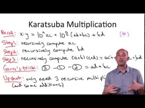
The Karatsuba Multiplication Algorithm
Karatsuba’s algorithm reduces the multiplication of two n-digit numbers to at most single-digit multiplications in general (and exactly when n is a power of 2). Although the familiar grade school algorithm for multiplying numbers is how we work through multiplication in our day-to-day lives, it’s slower () in comparison, but only on a computer, of course!
Here’s how the grade school algorithm looks: (The following slides have been taken from Tim Roughgarden’s notes. They serve as a good illustration. I hope he doesn’t mind my sharing them.)
…and this is how Karatsuba Multiplication works on the same problem:
A More General Treatment
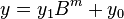
Let and be represented as -digit strings in some base. For any positive integer less than , one can write the two given numbers as
,
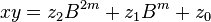
where and are less than . The product is then
where
These formulae require four multiplications, and were known to Charles Babbage. Karatsuba observed that can be computed in only three multiplications, at the cost of a few extra additions. With and as before we can calculate
which holds since
A more efficient implementation of Karatsuba multiplication can be set as , where .
Example
To compute the product of 12345 and 6789, choose B = 10 and m = 3. Then we decompose the input operands using the resulting base (Bm = 1000), as:
12345 = 12 · 1000 + 345
6789 = 6 · 1000 + 789
Only three multiplications, which operate on smaller integers, are used to compute three partial results:
We get the result by just adding these three partial results, shifted accordingly (and then taking carries into account by decomposing these three inputs in base 1000 like for the input operands):
This file contains hidden or bidirectional Unicode text that may be interpreted or compiled differently than what appears below. To review, open the file in an editor that reveals hidden Unicode characters.
Learn more about bidirectional Unicode characters
This file contains hidden or bidirectional Unicode text that may be interpreted or compiled differently than what appears below. To review, open the file in an editor that reveals hidden Unicode characters.
Learn more about bidirectional Unicode characters
It has been 3 years since I have steered my interests towards Machine Learning. I had just graduated from college with a Bachelor of Engineering in Electronics and Communication Engineering. Which is, other way of saying that I was:
a toddler in programming.
little / no knowledge of algorithms.
studied engineering math, but it was rusty.
no knowledge of modern optimization.
zero knowledge of statistical inference.
I think, most of it is true for many engineering graduates (especially, in India !). Unless, you studied mathematics and computing for undergrad.
Lucky for me, I had a great mentor and lot of online materials on these topics. This post will list many such materials I found useful, while I was learning it the hard way !
All the courses that I’m listing below have homework assignments. Make sure you work through each one of them.
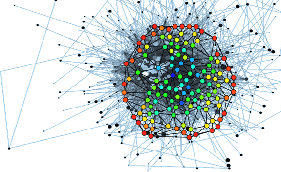
Yet another exciting math problem that requires an algorithmic approach to arrive at a quick solution! There is a pen-paper approach to it too, but this post assumes we’re more interested in discussing the programming angle.
Working clockwise, and starting from the group of three with the numerically lowest external node (4,3,2 in this example), each solution can be described uniquely. For example, the above solution can be described by the set: 4,3,2; 6,2,1; 5,1,3.
It is possible to complete the ring with four different totals: 9, 10, 11, and 12. There are eight solutions in total.
Total Solution Set: 9 4,2,3; 5,3,1; 6,1,2 9 4,3,2; 6,2,1; 5,1,3 10 2,3,5; 4,5,1; 6,1,3 10 2,5,3; 6,3,1; 4,1,5 11 1,4,6; 3,6,2; 5,2,4 11 1,6,4; 5,4,2; 3,2,6 12 1,5,6; 2,6,4; 3,4,5 12 1,6,5; 3,5,4; 2,4,6
By concatenating each group it is possible to form 9-digit strings; the maximum string for a 3-gon ring is432621513.
Problem
Using the numbers 1 to 10, and depending on arrangements, it is possible to form 16-and 17-digit strings. What is the maximum 16-digit string for a “magic” 5-gon ring?
Algorithm
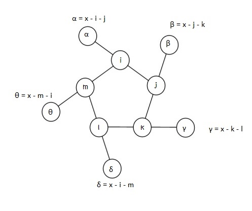
In attempting this problem, I choose to label the 5 inner nodes as i, j, k, l, and m. α, β, γ, δ, and θ being the corresponding outer nodes.
Let x be the sum total of each triplet line, i.e.,
x = α + i + j = β + j + k = γ + k + l = δ + l + m = θ + m + i
First Observation:
For the string to be 16-digits, 10 has to be in the outer ring, as each number in the inner ring is included in the string twice. Next, we fill the inner ring in an iterative manner.
Second Observation:
There 9 numbers to choose from for the inner ring — 1, 2, 3, 4, 5, 6, 7, 8 and 9.
5 have to be chosen. This can be done in 9C5 = 126 ways.
According to circular permutation, if there are n distinct numbers to be arranged in a circle, this can be done in (n-1)! ways, where (n-1)!= (n-1).(n-2).(n-3)…3.2.1. So 5 distinct numbers can be arranged in 4! permutations, i.e., in 24 ways around a circle, or pentagonal ring, to be more precise.
So in all, this problem can be solved in 126×24 =3024 iterations.
Third Observation:
For every possible permutation of an inner-ring arrangement, there can be one or more values of x(triplet line-sum) that serve as a possible contenders for a “magic”string whose triplets add up to the same number, x. To ensure this, we only need that the values of αthroughθ of the outer ring are distinct, different from the inner ring, with the greatest of these equal to 10.
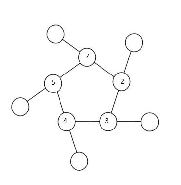
Depending on the relative positioning of the numbers in the inner ring, one can narrow the range of x-values one might have to check for each permutation. To zero-down on such a range, let’s look at an example. Shown in the figure below is a randomly chosen permutation of number in the inner ring – 7, 2, 3, 4 and 5, in that order.
So 10, 9, 8, 6 and 1 must fill the outer circle. It’s easy to notice that the 5, 7 pair is the greatest adjacent pair. So whatever x is, it has to be at least5 + 7 + 1 = 13 (1 being the smallest number of the outer ring). Likewise, 2, 3 is the smallest adjacent pair, so whatever x is, it can’t be any more than 2 + 3+ 10 = 15 (10 being the largest number of the outer ring). This leaves us with a narrow range of x-values to check – 13, 14 and 15.
Next, we arrange the 5 triplets in clock-wise direction starting with the triplet with the smallest number in the outer ring to form a candidate string. This exercise when done for each of the 3024permutations will shortlist a range of candidates, of which, the maximum is chosen.
That’s all there is to the problem!
Here’s the Python Code. It executes in about a tenth of a second!
This file contains hidden or bidirectional Unicode text that may be interpreted or compiled differently than what appears below. To review, open the file in an editor that reveals hidden Unicode characters.
Learn more about bidirectional Unicode characters


 single-digit multiplications in general (and exactly
  when n is a power of 2). Although the familiar grade school algorithm for multiplying numbers is how we work through multiplication in our day-to-day lives, it’s slower (
 ) in comparison, but only on a computer, of course!


 and
and  be represented as
  -digit strings in some
  . For any positive integer
  less than
 ,
, and
and  are less than
  . The product is then


 can be computed in only three multiplications, at the cost of a few extra additions. With
  and
and  as before we can calculate

 , where
  .
.