|
### Linear Regression Using lm() ---------------------------------------- |
|
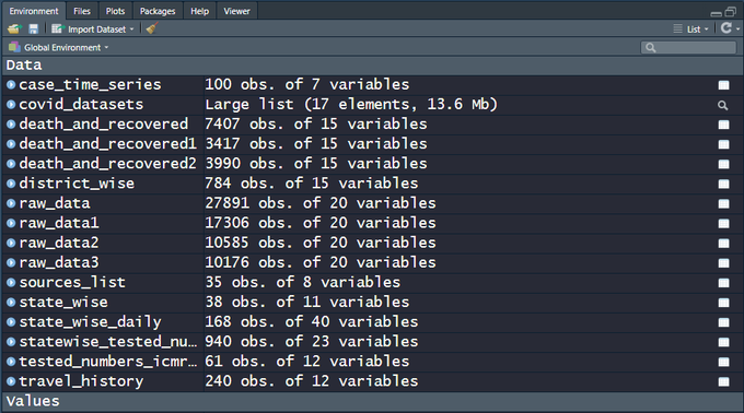
data("swiss") |
|
dat <- swiss |
|
linear_model <- lm(Fertility ~ ., data = dat) |
|
summary(linear_model) |
|
|
|
|
|
# Call: |
|
# lm(formula = Fertility ~ ., data = dat) |
|
# |
|
# Residuals: |
|
# Min 1Q Median 3Q Max |
|
# -15.2743 -5.2617 0.5032 4.1198 15.3213 |
|
# |
|
# Coefficients: |
|
# Estimate Std. Error t value Pr(>|t|) |
|
# (Intercept) 66.91518 10.70604 6.250 1.91e-07 *** |
|
# Agriculture -0.17211 0.07030 -2.448 0.01873 * |
|
# Examination -0.25801 0.25388 -1.016 0.31546 |
|
# Education -0.87094 0.18303 -4.758 2.43e-05 *** |
|
# Catholic 0.10412 0.03526 2.953 0.00519 ** |
|
# Infant.Mortality 1.07705 0.38172 2.822 0.00734 ** |
|
# --- |
|
# Signif. codes: 0 ‘***’ 0.001 ‘**’ 0.01 ‘*’ 0.05 ‘.’ 0.1 ‘ ’ 1 |
|
# |
|
# Residual standard error: 7.165 on 41 degrees of freedom |
|
# Multiple R-squared: 0.7067, Adjusted R-squared: 0.671 |
|
# F-statistic: 19.76 on 5 and 41 DF, p-value: 5.594e-10 |
|
|
|
|
|
### Using Linear Algebra ------------------------------------------------ |
|
|
|
y <- matrix(dat$Fertility, nrow = nrow(dat)) |
|
X <- cbind(1, as.matrix(x = dat[,-1])) |
|
colnames(X)[1] <- "(Intercept)" |
|
|
|
# N x k matrix |
|
N <- nrow(X) |
|
k <- ncol(X) - 1 # number of predictor variables (ergo, excluding Intercept column) |
|
|
|
# Estimated Regression Coefficients |
|
beta_hat <- solve(t(X)%*%X)%*%(t(X)%*%y) |
|
|
|
# Variance of outcome variable = Variance of residuals |
|
sigma_sq <- residual_variance <- (N-k-1)^-1 * sum((y - X %*% beta_hat)^2) |
|
residual_std_error <- sqrt(residual_variance) |
|
|
|
# Variance and Std. Error of estimated coefficients of the linear model |
|
var_betaHat <- sigma_sq * solve(t(X) %*% X) |
|
coeff_std_errors <- sqrt(diag(var_betaHat)) |
|
|
|
# t values of estimates are ratio of estimated coefficients to std. errors |
|
t_values <- beta_hat / coeff_std_errors |
|
|
|
# p-values of t-statistics of estimated coefficeints |
|
p_values_tstat <- 2 * pt(abs(t_values), N-k, lower.tail = FALSE) |
|
|
|
# assigning R's significance codes to obtained p-values |
|
signif_codes_match <- function(x){ |
|
ifelse(x <= 0.001,"***", |
|
ifelse(x <= 0.01,"**", |
|
ifelse(x < 0.05,"*", |
|
ifelse(x < 0.1,"."," ")))) |
|
|
|
} |
|
signif_codes <- sapply(p_values_tstat, signif_codes_match) |
|
|
|
# R-squared and Adjusted R-squared (refer any econometrics / statistics textbook) |
|
R_sq <- 1 - (N-k-1)*residual_variance / (N*mean((y - mean(y))^2)) |
|
R_sq_adj <- 1 - residual_variance / ((N/(N-1))*mean((y - mean(y))^2)) |
|
|
|
# Residual sum of squares (RSS) for the full model |
|
RSS <- (N-k-1)*residual_variance |
|
# RSS for the partial model with only intercept (equal to mean), ergo, TSS |
|
RSS0 <- TSS <- sum((y - mean(y))^2) |
|
|
|
# F statistic based on RSS for full and partial models |
|
# k = degress of freedom of partial model |
|
# N - k - 1 = degress of freedom of full model |
|
F_stat <- ((RSS0 - RSS)/k) / (RSS/(N-k-1)) |
|
|
|
# p-values of the F statistic |
|
p_value_F_stat <- pf(F_stat, df1 = k, df2 = N-k-1, lower.tail = FALSE) |
|
|
|
# stitch the main results toghether |
|
lm_results <- as.data.frame(cbind(beta_hat, coeff_std_errors, |
|
t_values, p_values_tstat, signif_codes)) |
|
colnames(lm_results) <- c("Estimate","Std. Error","t value","Pr(>|t|)","") |
|
|
|
|
|
### Print out results of all relevant calcualtions ----------------------- |
|
|
|
|
|
print(lm_results) |
|
cat("Residual standard error: ", |
|
round(residual_std_error, digits = 3), |
|
" on ",N-k-1," degrees of freedom", |
|
"\nMultiple R-squared: ",R_sq," Adjusted R-squared: ",R_sq_adj, |
|
"\nF-statistic: ",F_stat, " on ",k-1," and ",N-k-1, |
|
" DF, p-value: ", p_value_F_stat,"\n") |
|
|
|
# Estimate Std. Error t value Pr(>|t|) |
|
# (Intercept) 66.9151816789654 10.7060375853301 6.25022854119771 1.73336561301153e-07 *** |
|
# Agriculture -0.172113970941457 0.0703039231786469 -2.44814177018405 0.0186186100433133 * |
|
# Examination -0.258008239834722 0.253878200892098 -1.01626779663678 0.315320687313066 |
|
# Education -0.870940062939429 0.183028601571259 -4.75849159892283 2.3228265226988e-05 *** |
|
# Catholic 0.104115330743766 0.035257852536169 2.95296858017545 0.00513556154915653 ** |
|
# Infant.Mortality 1.07704814069103 0.381719650858061 2.82156849475775 0.00726899472564356 ** |
|
|
|
# Residual standard error: 7.165 on 41 degrees of freedom |
|
# Multiple R-squared: 0.706735 Adjusted R-squared: 0.670971 |
|
# F-statistic: 19.76106 on 4 and 41 DF, p-value: 5.593799e-10 |
|
|
|
|
 ,
,
 is the
  outcome variable and
  is the
  data matrix of independent predictor variables (including a vector of ones corresponding to the intercept). The ordinary least squares (OLS) estimate for the vector of coefficients
  is:
is:


 and with these, one can compute the t-statistics and their corresponding p-values.
 – for the full model with all predictors
 – for the partial model (
![\mathbf{y} = \mathbf{\mu} + \mathbf{\nu}; \mathbf{\mu} = \mathop{\mathbb{E}}[\mathbf{y}]; \mathbf{\nu} \sim N(0, \sigma_0^2 \mathbf{I})](https://s0.wp.com/latex.php?latex=%5Cmathbf%7By%7D+%3D+%5Cmathbf%7B%5Cmu%7D+%2B+%5Cmathbf%7B%5Cnu%7D%3B+%5Cmathbf%7B%5Cmu%7D+%3D+%5Cmathop%7B%5Cmathbb%7BE%7D%7D%5B%5Cmathbf%7By%7D%5D%3B+%5Cmathbf%7B%5Cnu%7D+%5Csim+N%280%2C+%5Csigma_0%5E2+%5Cmathbf%7BI%7D%29+&bg=f5f6f7&fg=444444&s=1&c=20201002) ) with the outcome observed mean as estimated outcome
) with the outcome observed mean as estimated outcome
