I got really interested in Computational Probability and Inference (6.008.1x) for the following reasons:
- I love probability and have solved countless problems on probability ever since I learned math
- …and yet I’ve never coded up probabilistic models!
- The assignments and project work for this course are to be implemented in Python!
You don’t need to have prior experience in either probability or inference, but you should be comfortable with basic Python programming and calculus.
WHAT YOU’LL LEARN
– Basic discrete probability theory
– Graphical models as a data structure for representing probability distributions
– Algorithms for prediction and inference
– How to model real-world problems in terms of probabilistic inference
The course started on September 12, is 12-weeks long and is structured in the following manner:
Week 1 (9/12 – 9/16): Introduction to probability and computation
A first look at basic discrete probability, how to interpret it, what probability spaces and random variables are, and how to code these up and do basic simulations and visualizations.
Week 2 (9/19 – 9/23): Incorporating observations
Incorporating observations using jointly distributed random variables and using events. Three classic probability puzzles are presented to help elucidate how to interpret probability: Simpson’s paradox, Monty Hall, boy or girl paradox.
Week 3 (9/26 – 9/30): Introduction to inference, structure in distributions, and information measures
The product rule and inference with Bayes’ theorem. Independence: A structure in distributions. Measures of randomness: entropy and information divergence. Mutual information.
Week 4 (10/3 – 10/7): Expectations, and driving to infinity in modeling uncertainty
Expected values of random variables. Classic puzzle: the two envelope problem. Probability spaces and random variables that take on a countably infinite number of values and inference with these random variables.
Week 5 (10/10 – 10/14): Efficient representations of probability distributions on a computer
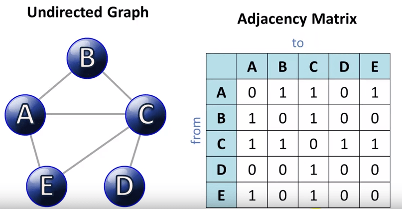
Introduction to undirected graphical models as a data structure for representing probability distributions and the benefits/drawbacks of these graphical models. Incorporating observations with graphical models.
Week 6 (10/17 – 10/21): Inference with graphical models, part I
Computing marginal distributions with graphical models in undirected graphical models including hidden Markov models..
Week 7 (10/24 – 10/28): Inference with graphical models, part II
Computing most probable configurations with graphical models including hidden Markov models.
Week 8 (10/31 – 11/4): Introduction to learning probability distributions
Learning an underlying unknown probability distribution from observations using maximum likelihood. Three examples: estimating the bias of a coin, the German tank problem, and email spam detection.
Week 9 (11/7 – 11/11): Parameter estimation in graphical models
Given the graph structure of an undirected graphical model, we examine how to estimate all the tables associated with the graphical model.
Week 10 (11/14 – 11/18): Model selection with information theory
Learning both the graph structure and the tables of an undirected graphical model with the help of information theory. Mutual information of random variables.
Week 11 (11/21 – 11/25): Final project
Final project assigned
Week 12 (11/28 – 12/2): Final project
I’m SO taking this course. Hope this interests you as well!