I am auditing this course currently and just completed its 2nd assignment. It’s probably one of the best courses out there to learn R in a way that you go beyond the syntax with an objective in mind – to do analytics and run machine learning algorithms to derive insight from data. This course is different from machine learning courses by say, Andrew Ng in that this course won’t focus on coding the algorithm and rather would emphasize on diving right into the implementation of those algorithms using libraries that the R programming language already equips us with.
Take a look at the course logistics. And hey, they’ve got a Kaggle competition!
There’s still time to enroll and grab a certificate (or simply audit). The course is offered once a year. I met a bunch of people who did well at a data hackathon I had gone to recently, who had learned the ropes in data science thanks to Analytics Edge.
Edit: This post is in its infancy. Work is still ongoing as far as deriving insight from the data is concerned. More content and economic insight is expected to be added to this post as and when progress is made in that direction.
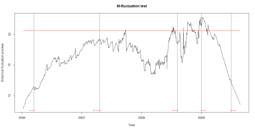
This is an attempt to detect structural breaks in China’s FX regime using Frenkel Wei regression methodology (this was later improved by Perron and Bai). I came up with the motivation to check for these structural breaks while attending a guest lecture on FX regimes by Dr. Ajay Shah delivered at IGIDR. This is work that I and two other classmates are working on as a term paper project under the supervision of Dr. Rajeswari Sengupta.
The code below can be replicated and run as is, to get same results.
This file contains hidden or bidirectional Unicode text that may be interpreted or compiled differently than what appears below. To review, open the file in an editor that reveals hidden Unicode characters.
Learn more about bidirectional Unicode characters
As can be seen in the figure below, the structural breaks correspond to the vertical bars. We are still working on understanding the motivations of China’s central bank in varying the degree of the managed float exchange rate.
EDIT (May 16, 2016):
The code above uses data provided by the package itself. If you wished to replicate this analysis on data after 2010, you will have to use your own data. We used Quandl, which lets you get 10 premium datasets for free. An API key (for only 10 calls on premium datasets) is provided if you register there. Foreign exchange rate data (2000 onward till date) apparently, is premium data. You can find these here.
Here are the (partial) results and code to work the same methodology on the data from 2010 to 2016:
This file contains hidden or bidirectional Unicode text that may be interpreted or compiled differently than what appears below. To review, open the file in an editor that reveals hidden Unicode characters.
Learn more about bidirectional Unicode characters
We got breaks in 2010 and in 2015 (when China’s stock markets crashed). We would have hoped for more breaks (we can still get them), but that would depend on the parameters chosen for our regression.
Deep learning became a hot topic in machine learning in the last 3-4 years (see inset below) and recently, Google released TensorFlow (a Python based deep learning toolkit) as an open source project to bring deep learning to everyone.
Interest in the Google search term Deep Learning over time
If you have wanted to get your hands dirty with TensorFlow or needed more direction with that, here’s some good news – Google is offering an open MOOC on deep learning methods using TensorFlow here. This course has been developed with Vincent Vanhoucke, Principal Scientist at Google, and technical lead in the Google Brain team. However, this is an intermediate to advanced level course and assumes you have taken a first course in machine learning, or that you are at least familiar with supervised learning methods.
Google’s overall goal in designing this course is to provide the machine learning enthusiast a rapid and direct path to solving real and interesting problems with deep learning techniques.
This happens to be my 50th blog post – and my blog is 8 months old.
🙂
This post is the third and last post in in a series of posts (Part 1 – Part 2) on data manipulation with dlpyr. Note that the objects in the code may have been defined in earlier posts and the code in this post is in continuation with code from the earlier posts.
Although datasets can be manipulated in sophisticated ways by linking the 5 verbs of dplyr in conjunction, linking verbs together can be a bit verbose.
Creating multiple objects, especially when working on a large dataset can slow you down in your analysis. Chaining functions directly together into one line of code is difficult to read. This is sometimes called the Dagwood sandwich problem: you have too much filling (too many long arguments) between your slices of bread (parentheses). Functions and arguments get further and further apart.
The %>% operator allows you to extract the first argument of a function from the arguments list and put it in front of it, thus solving the Dagwood sandwich problem.
This file contains hidden or bidirectional Unicode text that may be interpreted or compiled differently than what appears below. To review, open the file in an editor that reveals hidden Unicode characters.
Learn more about bidirectional Unicode characters
group_by() defines groups within a data set. Its influence becomes clear when calling summarise() on a grouped dataset. Summarizing statistics are calculated for the different groups separately.
This file contains hidden or bidirectional Unicode text that may be interpreted or compiled differently than what appears below. To review, open the file in an editor that reveals hidden Unicode characters.
Learn more about bidirectional Unicode characters
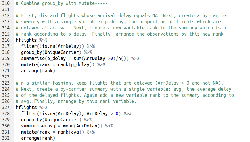
group_by() can also be combined with mutate(). When you mutate grouped data, mutate() will calculate the new variables independently for each group. This is particularly useful when mutate() uses the rank() function, that calculates within group rankings. rank() takes a group of values and calculates the rank of each value within the group, e.g.
rank(c(21, 22, 24, 23))
has output
[1] 1 2 4 3
As with arrange(), rank() ranks values from the largest to the smallest and this behaviour can be reversed with the desc() function.
This file contains hidden or bidirectional Unicode text that may be interpreted or compiled differently than what appears below. To review, open the file in an editor that reveals hidden Unicode characters.
Learn more about bidirectional Unicode characters
So after 8 months of playing around with R and Python and blog post after blog post, I found myself finally hacking away at a problem set from the 17th storey of the Hindustan Times building at Connaught Place. I had entered my first ever data science hackathon conducted by Analytics Vidhya, a pioneer in analytics learning in India. Pizzas and Pepsi were on the house. Like any predictive analysis hackathon, this one accepted unlimited entries till submission time. It was from 2pm to 4:30pm today – 2.5 hours, of which I ended up wasting 1.5 hours trying to make my first submission which encountered submission error after submission error until the problem was fixed finally post lunch. I had 1 hour to try my best. It wasn’t the best performance, but I thought of blogging this experience anyway, as a reminder of the work that awaits me. I want to be the one winning prize money at the end of the day.
Note that this post is in continuation with Part 1 of this series of posts on data manipulation with dplyr in R. The code in this post carries forward from the variables / objects defined in Part 1.
In the previous post, I talked about how dplyr provides a grammar of sorts to manipulate data, and consists of 5 verbs to do so:
The 5 verbs of dplyr select – removes columns from a dataset filter – removes rows from a dataset arrange – reorders rows in a dataset mutate – uses the data to build new columns and values summarize – calculates summary statistics
I went on to discuss examples using select() and mutate(). Let’s now talk about filter(). R comes with a set of logical operators that you can use inside filter(). These operators are: x < y,TRUE if x is less than y x <= y, TRUE if x is less than or equal to y x == y, TRUE if x equals y x != y, TRUE if x does not equal y x >= y, TRUE if x is greater than or equal to y x > y, TRUE if x is greater than y x %in% c(a, b, c), TRUE if x is in the vector c(a, b, c)
The following call, for example, filters df such that only the observations where the variable a is greater than the variable b: filter(df, a > b)
This file contains hidden or bidirectional Unicode text that may be interpreted or compiled differently than what appears below. To review, open the file in an editor that reveals hidden Unicode characters.
Learn more about bidirectional Unicode characters
Combining tests using boolean operators
R also comes with a set of boolean operators that you can use to combine multiple logical tests into a single test. These include & (and), | (or), and ! (not). Instead of using the & operator, you can also pass several logical tests to filter(), separated by commas. The following calls equivalent:
filter(df, a > b & c > d) filter(df, a > b, c > d)
The is.na() will also come in handy very often. This expression, for example, keeps the observations in df for which the variable x is not NA:
filter(df, !is.na(x))
This file contains hidden or bidirectional Unicode text that may be interpreted or compiled differently than what appears below. To review, open the file in an editor that reveals hidden Unicode characters.
Learn more about bidirectional Unicode characters
This file contains hidden or bidirectional Unicode text that may be interpreted or compiled differently than what appears below. To review, open the file in an editor that reveals hidden Unicode characters.
Learn more about bidirectional Unicode characters
Arranging Data arrange() can be used to rearrange rows according to any type of data. If you pass arrange() a character variable, R will rearrange the rows in alphabetical order according to values of the variable. If you pass a factor variable, R will rearrange the rows according to the order of the levels in your factor (running levels() on the variable reveals this order).
By default, arrange() arranges the rows from smallest to largest. Rows with the smallest value of the variable will appear at the top of the data set. You can reverse this behaviour with the desc() function. arrange() will reorder the rows from largest to smallest values of a variable if you wrap the variable name in desc() before passing it to arrange()
This file contains hidden or bidirectional Unicode text that may be interpreted or compiled differently than what appears below. To review, open the file in an editor that reveals hidden Unicode characters.
Learn more about bidirectional Unicode characters
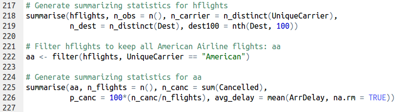
summarise(), the last of the 5 verbs, follows the same syntax as mutate(), but the resulting dataset consists of a single row instead of an entire new column in the case of mutate().
In contrast to the four other data manipulation functions, summarise() does not return an altered copy of the dataset it is summarizing; instead, it builds a new dataset that contains only the summarizing statistics.
Note:summarise() and summarize() both work the same!
You can use any function you like in summarise(), so long as the function can take a vector of data and return a single number. R contains many aggregating functions. Here are some of the most useful:
min(x) – minimum value of vector x. max(x) – maximum value of vector x. mean(x) – mean value of vector x. median(x) – median value of vector x. quantile(x, p) – pth quantile of vector x. sd(x) – standard deviation of vector x. var(x) – variance of vector x. IQR(x) – Inter Quartile Range (IQR) of vector x. diff(range(x)) – total range of vector x.
This file contains hidden or bidirectional Unicode text that may be interpreted or compiled differently than what appears below. To review, open the file in an editor that reveals hidden Unicode characters.
Learn more about bidirectional Unicode characters
dplyr provides several helpful aggregate functions of its own, in addition to the ones that are already defined in R. These include:
first(x) – The first element of vector x. last(x) – The last element of vector x. nth(x, n) – The nth element of vector x. n() – The number of rows in the data.frame or group of observations that summarise() describes. n_distinct(x) – The number of unique values in vector x
This file contains hidden or bidirectional Unicode text that may be interpreted or compiled differently than what appears below. To review, open the file in an editor that reveals hidden Unicode characters.
Learn more about bidirectional Unicode characters
This would be it for Part-2 of this series of posts on data manipulation with dplyr. Part 3 would focus on the pipe operator, Group_by and working with databases.
dplyr is one of the packages in R that makes R so loved by data scientists. It has three main goals:
Identify the most important data manipulation tools needed for data analysis and make them easy to use in R.
Provide blazing fast performance for in-memory data by writing key pieces of code in C++.
Use the same code interface to work with data no matter where it’s stored, whether in a data frame, a data table or database.
Introduction to the dplyr package and the tbl class
This post is mostly about code. If you’re interested in learning dplyr I recommend you type in the commands line by line on the R console to see first hand what’s happening.
This file contains hidden or bidirectional Unicode text that may be interpreted or compiled differently than what appears below. To review, open the file in an editor that reveals hidden Unicode characters.
Learn more about bidirectional Unicode characters
Select and mutate dplyr provides grammar for data manipulation apart from providing data structure. The grammar is built around 5 functions (also referred to as verbs) that do the basic tasks of data manipulation.
The 5 verbs of dplyr select – removes columns from a dataset filter – removes rows from a dataset arrange – reorders rows in a dataset mutate – uses the data to build new columns and values summarize – calculates summary statistics
dplyr functions do not change the dataset. They return a new copy of the dataset to use.
To answer the simple question whether flight delays tend to shrink or grow during a flight, we can safely discard a lot of the variables of each flight. To select only the ones that matter, we can use select()
This file contains hidden or bidirectional Unicode text that may be interpreted or compiled differently than what appears below. To review, open the file in an editor that reveals hidden Unicode characters.
Learn more about bidirectional Unicode characters
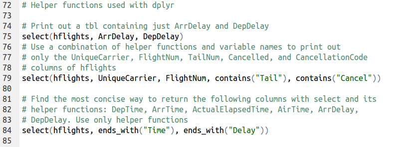
dplyr comes with a set of helper functions that can help you select variables. These functions find groups of variables to select, based on their names. Each of these works only when used inside of select()
starts_with(“X”): every name that starts with “X”
ends_with(“X”): every name that ends with “X”
contains(“X”): every name that contains “X”
matches(“X”): every name that matches “X”, where “X” can be a regular expression
num_range(“x”, 1:5): the variables named x01, x02, x03, x04 and x05
one_of(x): every name that appears in x, which should be a character vector
This file contains hidden or bidirectional Unicode text that may be interpreted or compiled differently than what appears below. To review, open the file in an editor that reveals hidden Unicode characters.
Learn more about bidirectional Unicode characters
In order to appreciate the usefulness of dplyr, here are some comparisons between base R and dplyr
This file contains hidden or bidirectional Unicode text that may be interpreted or compiled differently than what appears below. To review, open the file in an editor that reveals hidden Unicode characters.
Learn more about bidirectional Unicode characters
mutate() is the second of the five data manipulation functions. mutate() creates new columns which are added to a copy of the dataset.
This file contains hidden or bidirectional Unicode text that may be interpreted or compiled differently than what appears below. To review, open the file in an editor that reveals hidden Unicode characters.
Learn more about bidirectional Unicode characters
So far we have added variables to hflights one at a time, but we can also use mutate() to add multiple variables at once.
This file contains hidden or bidirectional Unicode text that may be interpreted or compiled differently than what appears below. To review, open the file in an editor that reveals hidden Unicode characters.
Learn more about bidirectional Unicode characters
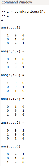
I have been doing Gilbert Strang’s linear algebra assignments, some of which require you to write short scripts in MatLab, though I use GNU Octave (which is kind of like a free MatLab). I was trying out this problem:
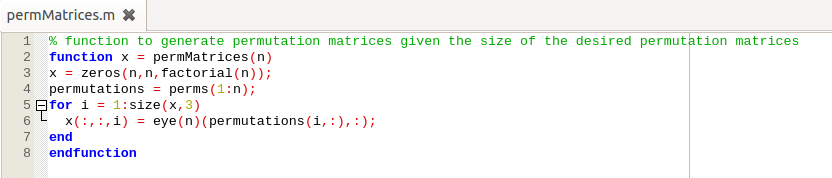
To solve this quickly, it would have been nice to have a function that would give a list of permutation matrices for every n-sized square matrix, but there was none in Octave, so I wrote a function permMatrices which creates a list of permutation matrices for a square matrix of size n.
This file contains hidden or bidirectional Unicode text that may be interpreted or compiled differently than what appears below. To review, open the file in an editor that reveals hidden Unicode characters.
Learn more about bidirectional Unicode characters
The MatLab / Octave code to solve this problem is shown below:
This file contains hidden or bidirectional Unicode text that may be interpreted or compiled differently than what appears below. To review, open the file in an editor that reveals hidden Unicode characters.
Learn more about bidirectional Unicode characters
On January 12, 2016, Stanford University professors Trevor Hastie and Rob Tibshirani will offer the 3rd iteration of Statistical Learning, a MOOC which first began in January 2014, and has become quite a popular course among data scientists. It is a great place to learn statistical learning (machine learning) methods using the R programming language. For a quick course on R, check this out – Introduction to R Programming
Slides and videos for Statistical Learning MOOC by Hastie and Tibshirani available separately here. Slides and video tutorials related to this book by Abass Al Sharif can be downloaded here.
The course covers the following book which is available for free as a PDF copy.
Logistics and Effort:
Rough Outline of Schedule (based on last year’s course offering):
Week 1: Introduction and Overview of Statistical Learning (Chapters 1-2) Week 2: Linear Regression (Chapter 3) Week 3: Classification (Chapter 4) Week 4: Resampling Methods (Chapter 5) Week 5: Linear Model Selection and Regularization (Chapter 6) Week 6: Moving Beyond Linearity (Chapter 7) Week 7: Tree-based Methods (Chapter 8) Week 8: Support Vector Machines (Chapter 9) Week 9: Unsupervised Learning (Chapter 10)
Prerequisites: First courses in statistics, linear algebra, and computing.
I found myself stuck on this problem recently. I must confess, I lost a couple of hours trying to get to figure the logic for this one. Here’s the problem:
I’ve written 2 functions to solve this problem. The first one I used for smaller N, say N < 30 and the second one for N > 30. The second function is elegant, and it relies on the mathematical property that if a number N is not divisible by 3, it could either leave a remainder 1 or 2.
If it leaves a remainder 2, then subtracting 5 once would make the number divisible by 3. If it leaves a remainder 1, then subtracting 5 twice would make the number divisible by 3.
We subtract 5 from N iteratively and attempt to divide N into 2 parts, one divisible by 3 and the other divisible by 5. We want the part that is divisible by 3 to be the larger part, so that the associated Decent Number is the largest possible. This explanation might seem obtuse, but if you get pen down on paper, you’ll understand what I mean.


 To solve this quickly, it would have been nice to have a function that would give a list of permutation matrices for every n-sized square matrix, but there was none in Octave, so I wrote a function