Author: Anirudh

  • Supplementary Material to Andrew Ng’s Machine Learning MOOC

    Supplementary Material to Andrew Ng’s Machine Learning MOOC

    Although the lecture videos and lecture notes from Andrew Ng‘s Coursera MOOC are sufficient for the online version of the course, if you’re interested in more mathematical stuff or want to be challenged further, you can go through the following notes and problem sets from CS 229, a 10-week course that he teaches at Stanford (which also happens to be the most enrolled course on campus). It’s not hard to end up with a 100% score on his MOOC which is obviously a (much) watered down version of the course he teaches at Stanford, at least in terms of difficulty. If you don’t believe me, just have a go at the problem sets from the links below.

    Lecture Notes

    Section Notes

    Handouts and Problem Sets

  • Solutions to Machine Learning Programming Assignments

    Solutions to Machine Learning Programming Assignments

    This post contains links to a bunch of code that I have written to complete Andrew Ng’s famous machine learning course which includes several interesting machine learning problems that needed to be solved using the Octave / Matlab programming language. I’m not sure I’d ever be programming in Octave after this course, but learning Octave just so that I could complete this course seemed worth the time and effort. I would usually work on the programming assignments on Sundays and spend several hours coding in Octave, telling myself that I would later replicate the exercises in Python.

    If you’ve taken this course and found some of the assignments hard to complete, I think it might not hurt to go check online on how a particular function was implemented. If you end up copying the entire code, it’s probably your loss in the long run. But then John Maynard Keynes once said, ‘In the long run we are all dead‘. Yeah, and we wonder why people call Economics the dismal science!

    Most people disregard Coursera’s feeble attempt at reigning in plagiarism by creating an Honor Code, precisely because this so-called code-of-conduct can be easily circumvented. I don’t mind posting solutions to a course’s programming assignments because GitHub is full to the brim with such content. Plus, it’s always good to read others’ code even if you implemented a function correctly. It helps understand the different ways of tackling a given programming problem.

    ex1
    ex2
    ex3
    ex4
    ex5
    ex6
    ex7
    ex8

    Enjoy!


  • Troubleshooting ‘Rattle’ (R library) Installation on Ubuntu

    Troubleshooting ‘Rattle’ (R library) Installation on Ubuntu

    This post pertains to Ubuntu / Debian users only.

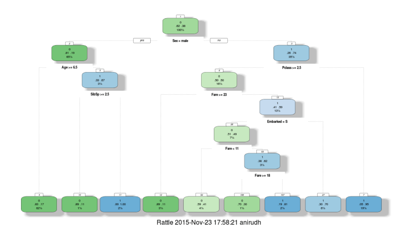
    rattle is a free graphical interface for data mining with R. I wanted to visualize decision trees and had to install this library.
    > install.packages('rattle')
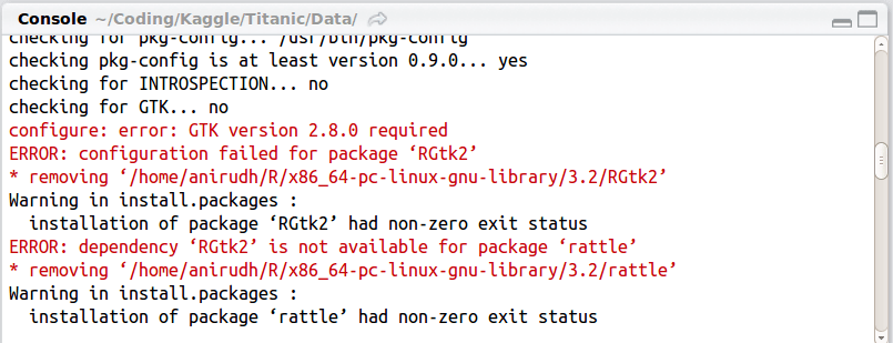
    got me the following error message:

    configure: error: GTK version 2.8.0 required
    ERROR: configuration failed for package ‘RGtk2’

    rattle_installationNonZeroExit

    This error occurs when attempting to install the RGtk2 package. The install is looking for the header files for GTK. Possibly they are not yet. Luckily the problem can be solved quite easily. Open Terminal (Ctrl + Alt + T) and type in the following commands:


    sudo apt-get update
    wajig install libgtk2.0-dev

    Go back and try installing rattle now with the same command as earlier. It should work. It did for me! As you can see below, decision trees are visualized lot better with rattle than if you used just rpart.

    rattle

  • Spot the Difference — It’s NumPy!

    Spot the Difference — It’s NumPy!

    My first brush with NumPy happened over writing a block of code to make a plot using pylab. ⇣


    pylab is part of matplotlib (in matplotlib.pylab) and tries to give you a MatLab like environment. matplotlib has a number of dependencies, among them numpy which it imports under the common alias np. scipy is not a dependency of matplotlib.


    I had a tuple (of lows and highs of temperature) of lengh 2 with 31 entries in each (the number of days in the month of July), parsed from this text file:

    Boston July Temperatures
    ————————-
    Day High Low
    ————
    1 91 70
    2 84 69
    3 86 68
    4 84 68
    5 83 70
    6 80 68
    7 86 73
    8 89 71
    9 84 67
    10 83 65
    11 80 66
    12 86 63
    13 90 69
    14 91 72
    15 91 72
    16 88 72
    17 97 76
    18 89 70
    19 74 66
    20 71 64
    21 74 61
    22 84 61
    23 86 66
    24 91 68
    25 83 65
    26 84 66
    27 79 64
    28 72 63
    29 73 64
    30 81 63
    31 73 63
    view raw julyTemps.txt hosted with ❤ by GitHub

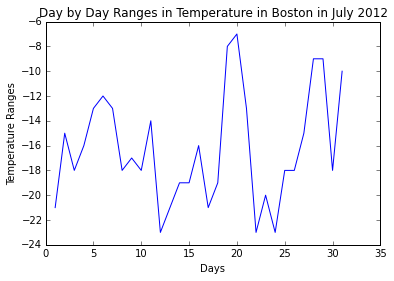
    Given below, are 2 sets of code that do the same thing; one without NumPy and the other with NumPy. They output the following graph using PyLab:

    differenceTemp

    Code without NumPy

    import pylab
    def loadfile():
    inFile = open('julyTemps.txt', 'r')
    high =[]; low = []
    for line in inFile:
    fields = line.split()
    if len(fields) < 3 or not fields[0].isdigit():
    pass
    else:
    high.append(int(fields[1]))
    low.append(int(fields[2]))
    return low, high
    def producePlot(lowTemps, highTemps):
    diffTemps = [highTemps[i] – lowTemps[i] for i in range(len(lowTemps))]
    pylab.title('Day by Day Ranges in Temperature in Boston in July 2012')
    pylab.xlabel('Days')
    pylab.ylabel('Temperature Ranges')
    return pylab.plot(range(1,32),diffTemps)
    producePlot(loadfile()[1], loadfile()[0])
    view raw withoutNumPy.py hosted with ❤ by GitHub

    Code with NumPy
    import pylab
    import numpy as np
    def loadFile():
    inFile = open('julyTemps.txt')
    high = [];vlow = []
    for line in inFile:
    fields = line.split()
    if len(fields) != 3 or 'Boston' == fields[0] or 'Day' == fields[0]:
    continue
    else:
    high.append(int(fields[1]))
    low.append(int(fields[2]))
    return (low, high)
    def producePlot(lowTemps, highTemps):
    diffTemps = list(np.array(highTemps) – np.array(lowTemps))
    pylab.plot(range(1,32), diffTemps)
    pylab.title('Day by Day Ranges in Temperature in Boston in July 2012')
    pylab.xlabel('Days')
    pylab.ylabel('Temperature Ranges')
    pylab.show()
    (low, high) = loadFile()
    producePlot(low, high)
    view raw withNumPy.py hosted with ❤ by GitHub

    The difference in code lies in how the variable diffTemps is calculated.

    diffTemps = list(np.array(highTemps) - np.array(lowTemps))
    

    seems more readable than

    diffTemps = [highTemps[i] - lowTemps[i] for i in range(len(lowTemps))]
    

    Notice how straight forward it is with NumPy. At the core of the NumPy package, is the ndarray object. This encapsulates n-dimensional arrays of homogeneous data types, with many operations being performed in compiled code for performance. element-by-element operations are the “default mode” when an ndarray is involved, but the element-by-element operation is speedily executed by pre-compiled C code.

  • MITx 6.00.2x Introduction to Computational Thinking and Data Science (Fall 2015)

    MITx 6.00.2x Introduction to Computational Thinking and Data Science (Fall 2015)

    MIT’s Fall 2015 iteration of 6.00.2x starts today. After an enriching learning experience with 6.00.1x, I have great expectations from this course. As the course website mildly puts it, 6.00.2x is an introduction to using computation to understand real-world phenomena. MIT OpenCourseware (OCW) mirroring the material covered in 6.00.1x and 6.00.2x can be found here.

    The course follows this book by John Guttag (who happens to be one of the instructors for this course). However, purchasing the book isn’t a necessity for this course.

    Introduction to Computation and Programming Using Python

    One thing I loved about 6.00.1x was its dedicated Facebook group, which gave a community / classroom-peergroup feel to the course. 6.00.2x also has a Facebook group. Here’s a sneak peak:

    descriptionUpdate

    The syllabus and schedule for this course is shown below. The course is spread out over 2 months which includes 7 weeks of lectures.

    MITx 6.00.2x Fall 2015 Course Calendar
    MITx 6.00.2x Fall 2015 Course Calendar

    The prerequisites for this course are pretty much covered in this set of tutorial videos that have been created by one of the TAs for 6.00.1x. If you’ve not taken 6.00.1x in the past, you can go through these videos (running time < 1hr) to judge whether or not to go ahead with 6.00.2x.

    So much for the update. Got work to do! 🙂

  • Funny Python

    Funny Python

    If a programming language is named after a sketch comedy troupe, one knows what to expect. Python IS a funny language with its own bag of surprises.

    pythonMonty
    Monty Python’s Flying Circus

    For instance, If you’ve just moved from a language such as C to Python and you’re missing curly braces (how can one not want whitespaces!!), and you try this:

    >>> from __future__ import braces

    from __future__ import braces
    Click Image for Larger View

    Or say, if you try importing this.

    >>> import this

    import this
    A sense of humour is required for proper interpretation

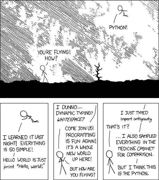
    Or if you ever wanted to know why XKCD’s Cueball left Perl for Python, you should know, that it was for gravity defying stunts that he couldn’t perform anywhere else. Just import antigravity!

    >>> import antigravity

    You’re led to this webcomic on your browser.

    import antigravity

    So the upshot is that you can get tickled and trolled by Python every now and then, keeping in line with its rich tradition of doing so (check out video below).

    Comedians!

  • Python to the Rescue

    Python to the Rescue

    Another journal-like entry

    Programming as a profession is only moderately interesting. It can be a good job, but you could make about the same money and be happier running a fast food joint. You’re much better off using code as your secret weapon in another profession.

    People who can code in the world of technology companies are a dime a dozen and get no respect. People who can code in biology, medicine, government, sociology, physics, history, and mathematics are respected and can do amazing things to advance those disciplines.

    Advice from an Old Programmer

    I was reading a paper today, written by MIT’s Esther Duflo, part of a homework assignment on a MOOC on development policy (Foundations of Development Policy: Advanced Development Economics) offered by Duflo and Abhijit Banerjee. So I opened the paper and started copying important lines from the PDF to a text editor to make notes. I could copy the text, but when I pasted it onto a text editor, it turned out to be gibberish (you can try it too!).

    For instance, instead of pasting

    Between 1973 and 1978 the Indonesian Government constructed over 61,000 primary schools throughout the county

    I got:

    Ehwzhhq 4<:6 dqg 4<:;/ wkh Lqgrqhvldq Jryhuqphqw frqv wuxfwhg ryhu 94/333 sulpdu| vfkrrov wkurxjkrxw wkh frxqwu|

    It was a good thing the cipher used for this text wasn’t too complicated. After some perusal, I found that ‘B’ became ‘E’, ‘e’ became ‘h’, ‘t’ became ‘w’ and so on. So I copied the entire content of the PDF to a text file and named the encrypted file estherDuflo.txt. I noticed that the encryption had been implemented only on the first 1475 lines. The remaining was plain English.

    So I wrote a Python script to decrypt the gibberish, rather than simply typing out my notes. It took 20 minutes writing the code and 8 ms to execute (of course!). I didn’t want to spend a lot of time ensuring a thorough decryption, so the result wasn’t perfect, but then I’m going to make do. I named the decrypted file estherDufloDecrypted.txt.

    Sample from the Encrypted File

    5U LL*?} @?_ w@MLh @h!i| L?ti^ i?Uit Lu 5U LL*
    L?t|h U|L? ? W?_L?it@G ,_i?Ui uhL4 @? N? t @* L*U)
    , Tih4i?|
    ,t| ih # L
    W
    Devwudfw
    Ehwzhhq 4<:6 dqg 4<:;/ wkh Lqgrqhvldq Jryhuqphqw frqvwuxfwhg ryhu 94/333 sulpdu|
    vfkrrov wkurxjkrxw wkh frxqwu|1 Wklv lv rqh ri wkh odujhvw vfkrro frqvwuxfwlrq surjudpv rq
    uhfrug1 L hydoxdwh wkh hhfw ri wklv surjudp rq hgxfdwlrq dqg zdjhv e| frpelqlqj glhuhqfhv
    dfurvv uhjlrqv lq wkh qxpehu ri vfkrrov frqvwuxfwhg zlwk glhuhqfhv dfurvv frkruwv lqgxfhg
    e| wkh wlplqj ri wkh surjudp1 Wkh hvwlpdwhv vxjjhvw wkdw wkh frqvwuxfwlrq ri sulpdu| vfkrrov
    ohg wr dq lqfuhdvh lq hgxfdwlrq dqg hduqlqjv1 Fkloguhq djhg 5 wr 9 lq 4<:7 uhfhlyhg 3145 wr
    314< pruh |hduv ri hgxfdwlrq iru hdfk vfkrro frqvwuxfwhg shu 4/333 fkloguhq lq wkhlu uhjlrq
    ri eluwk1 Xvlqj wkh yduldwlrqv lq vfkrrolqj jhqhudwhg e| wklv srolf| dv lqvwuxphqwdo yduldeohv
    iru wkh lpsdfw ri hgxfdwlrq rq zdjhv jhqhudwhv hvwlpdwhv ri hfrqrplf uhwxuqv wr hgxfdwlrq
    udqjlqj iurp 91; shufhqw wr 4319 shufhqw1 +MHO L5/ M64/ R48/ R55,
    Wkh txhvwlrq ri zkhwkhu lqyhvwphqw lq lqiudvwuxfwxuh lqfuhdvhv kxpdq fdslwdo dqg uhgxfhv
    sryhuw| kdv orqj ehhq d frqfhuq wr ghyhorsphqw hfrqrplvwv dqg srolf|pdnhuv1 Iru h{dpsoh/
    dydlodelolw| ri vfkrrolqj lqiudvwuxfwxuh kdv ehhq vkrzq wr eh srvlwlyho| fruuhodwhg zlwk frpsohwhg
    vfkrrolqj ru hquroophqw e| Qdqf| Elugvdoo +4<;8, lq xuedq Eud}lo/ Ghqqlv GhWud| +4<;;, dqg Ohh
    view raw estherDuflo.txt hosted with ❤ by GitHub

    My Code
    from string import *
    # create decipher dictionary
    l = letters[:26]
    decipher = "".join([l[(i+3)%26] for i in range(len(l))])
    decipher = dict(zip(decipher,l))
    # open and read encrypted text
    filename = 'estherDuflo.txt'
    f = open(filename, 'rw')
    lines = f.readlines()
    lines = [l[:-1] for l in lines]
    # use first 1475 lines only
    newlines = lines[:1475]
    # apply decryption on those 1475 lines
    decipheredLines = []
    for line in newlines:
    x = line.lower()
    s = []
    for letter in x:
    if letter in letters:
    s.append(decipher[letter])
    else:
    s.append(letter)
    s.append('\n')
    decipheredLines.append(''.join(s))
    # write deciphered text to new text file
    decipheredFile = 'estherDufloDeciphered.txt'
    df = open(decipheredFile, 'w')
    for line in decipheredLines:
    df.write("%s" % line)
    # close both text files
    f.close()
    df.close()
    view raw estherDuflo.py hosted with ❤ by GitHub

    Sample from the Decrypted File
    5r ii*?} @?_ t@jie @e!f| i?qf^ f?rfq ir 5r ii*
    i?q|e r|i? ? t?_i?fq@d ,_f?rf rei4 @? k? q @* i*r)
    , qfe4f?|
    ,q| fe # i
    t
    abstract
    between 4<:6 and 4<:;/ the indonesian government constructed over 94/333 primar|
    schools throughout the countr|1 this is one of the largest school construction programs on
    record1 i evaluate the eect of this program on education and wages b| combining dierences
    across regions in the number of schools constructed with dierences across cohorts induced
    b| the timing of the program1 the estimates suggest that the construction of primar| schools
    led to an increase in education and earnings1 children aged 5 to 9 in 4<:7 received 3145 to
    314< more |ears of education for each school constructed per 4/333 children in their region
    of birth1 using the variations in schooling generated b| this polic| as instrumental variables
    for the impact of education on wages generates estimates of economic returns to education
    ranging from 91; percent to 4319 percent1 +jel i5/ j64/ o48/ o55,
    the question of whether investment in infrastructure increases human capital and reduces
    povert| has long been a concern to development economists and polic|makers1 for e{ample/
    availabilit| of schooling infrastructure has been shown to be positivel| correlated with completed
    schooling or enrollment b| nanc| birdsall +4<;8, in urban bra}il/ dennis detra| +4<;;, and lee

  • Karatsuba Multiplication Algorithm – Python Code

    Karatsuba Multiplication Algorithm – Python Code

    Motivation for this blog post

    I’ve enrolled in Stanford Professor Tim Roughgarden’s Coursera MOOC on the design and analysis of algorithms, and while he covers the theory and intuition behind the algorithms in a surprising amount of detail, we’re left to implement them in a programming language of our choice.

    And I’m ging to post Python code for all the algorithms covered during the course!

    The Karatsuba Multiplication Algorithm

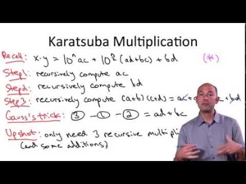
    Karatsuba’s algorithm reduces the multiplication of two n-digit numbers to at most  n^{\log_23}\approx n^{1.585} single-digit multiplications in general (and exactly n^{\log_23} when n is a power of 2). Although the familiar grade school algorithm for multiplying numbers is how we work through multiplication in our day-to-day lives, it’s slower (\Theta(n^2)\,\!) in comparison, but only on a computer, of course!

    Here’s how the grade school algorithm looks:
    (The following slides have been taken from Tim Roughgarden’s notes. They serve as a good illustration. I hope he doesn’t mind my sharing them.)

    gradeSchoolAlgorithm

    …and this is how Karatsuba Multiplication works on the same problem:

    exampleKaratsuba

    recursiveKaratsuba

    A More General Treatment

    Let x and y be represented as n-digit strings in some base B. For any positive integer m less than n, one can write the two given numbers as

    x = x_1B^m + x_0
    y = y_1B^m + y_0,

    where x_0 and y_0 are less than B^m. The product is then

    xy = (x_1B^m + x_0)(y_1B^m + y_0)
    xy = z_2B^{2m} + z_1B^m + z_0

    where

    z_2 = x_1y_1
    z_1 = x_1y_0 + x_0y_1
    z_0 = x_0y_0

    These formulae require four multiplications, and were known to Charles Babbage. Karatsuba observed that xy can be computed in only three multiplications, at the cost of a few extra additions. With z_0 and z_2 as before we can calculate

    z_1 = (x_1 + x_0)(y_1 + y_0) - z_2 - z_0

    which holds since

    z_1 = x_1y_0 + x_0y_1
    z_1 = (x_1 + x_0)(y_1 + y_0) - x_1y_1 - x_0y_0

    A more efficient implementation of Karatsuba multiplication can be set as xy = (b^2 + b)x_1y_1 - b(x_1 - x_0)(y_1 - y_0) + (b + 1)x_0y_0, where b = B^m.

    Example

    To compute the product of 12345 and 6789, choose B = 10 and m = 3. Then we decompose the input operands using the resulting base (Bm = 1000), as:

    12345 = 12 · 1000 + 345
    6789 = 6 · 1000 + 789

    Only three multiplications, which operate on smaller integers, are used to compute three partial results:

    z2 = 12 × 6 = 72
    z0 = 345 × 789 = 272205
    z1 = (12 + 345) × (6 + 789) − z2z0 = 357 × 795 − 72 − 272205 = 283815 − 72 − 272205 = 11538

    We get the result by just adding these three partial results, shifted accordingly (and then taking carries into account by decomposing these three inputs in base 1000 like for the input operands):

    result = z2 · B2m + z1 · Bm + z0, i.e.
    result = 72 · 10002 + 11538 · 1000 + 272205 = 83810205.

    Pseudocode and Python code

    procedure karatsuba(num1, num2)
    if (num1 < 10) or (num2 < 10)
    return num1*num2
    /* calculates the size of the numbers */
    m = max(size_base10(num1), size_base10(num2))
    m2 = m/2
    /* split the digit sequences about the middle */
    high1, low1 = split_at(num1, m2)
    high2, low2 = split_at(num2, m2)
    /* 3 calls made to numbers approximately half the size */
    z0 = karatsuba(low1,low2)
    z1 = karatsuba((low1+high1),(low2+high2))
    z2 = karatsuba(high1,high2)
    return (z2*10^(2*m2))+((z1-z2-z0)*10^(m2))+(z0)

    def karatsuba(x,y):
    """Function to multiply 2 numbers in a more efficient manner than the grade school algorithm"""
    if len(str(x)) == 1 or len(str(y)) == 1:
    return x*y
    else:
    n = max(len(str(x)),len(str(y)))
    nby2 = n / 2
    a = x / 10**(nby2)
    b = x % 10**(nby2)
    c = y / 10**(nby2)
    d = y % 10**(nby2)
    ac = karatsuba(a,c)
    bd = karatsuba(b,d)
    ad_plus_bc = karatsuba(a+b,c+d) – ac – bd
    # this little trick, writing n as 2*nby2 takes care of both even and odd n
    prod = ac * 10**(2*nby2) + (ad_plus_bc * 10**nby2) + bd
    return prod
    view raw karatsuba.py hosted with ❤ by GitHub

  • Getting Started with R on MIT’s 14.74x (Foundations of Development Policy)

    Getting Started with R on MIT’s 14.74x (Foundations of Development Policy)

    I noticed that a major grievance of many students enrolled in MIT‘s latest edX course on development policy (Foundations of Development Policy: Advanced Development Economics) was that there wasn’t enough done to get them going with the R assignments. I have posted the R code for the homework (past the deadline, of course) of the first 2 weeks, so that others get a hang of the level of R that might be needed to solve these assignments in the following weeks. I’m willing to help out those needing help getting up to speed with R required for this course. For specific queries, leave your message in the comments section.

    A great place to get spend time learning R before taking Foundations of Development Policy (14.74x) would be another edX course that’s been getting great reviews recently: Introduction to R Programming

    R Code for Home Work (Week 1)

    # set working directory to local directory where the data is kept
    setwd("~/IGIDR/Development Economics – MIT/Homework Assignment 01")
    # read the data
    wb_dev_ind = read.csv("wb_dev_ind.csv")
    # summarize data
    summary(wb_dev_ind)
    # Question 1
    # What is the Mean of GDP per capita? What is the standard deviation of GDP per capita?
    meanGDPperCapita = mean(wb_dev_ind$gdp_per_capita, na.rm = TRUE)
    print(round(meanGDPperCapita))
    sdGDPperCapita = sd(wb_dev_ind$gdp_per_capita, na.rm = TRUE)
    print(round(sdGDPperCapita))
    # Question 2
    # What is the mean illiteracy rate across all countries? What is the standard deviation?
    illiteracy_all = numeric(nrow(wb_dev_ind))
    wb_dev_ind$illiteracy_all = illiteracy_all
    wb_dev_ind$illiteracy_all = 100 – wb_dev_ind$literacy_all
    meanIlliteracy = mean(wb_dev_ind$illiteracy_all, na.rm = TRUE)
    print(round(meanIlliteracy))
    sdIlliteracy = sd(wb_dev_ind$illiteracy_all, na.rm = TRUE)
    print(round(sdIlliteracy))
    # Question 3
    # What is the mean infant mortality rate across all countries? What is the standard deviation?
    meanInfantMortality = mean(wb_dev_ind$infant_mortality, na.rm = TRUE)
    print(round(meanInfantMortality))
    sdInfantMortality = sd(wb_dev_ind$infant_mortality, na.rm = TRUE)
    print(round(sdInfantMortality))
    # Question 4
    # What is the mean male illiteracy rate? What is the mean female illiteracy rate?
    illiteracy_male = numeric(nrow(wb_dev_ind))
    wb_dev_ind$illiteracy_male = illiteracy_male
    wb_dev_ind$illiteracy_male = 100 – wb_dev_ind$literacy_male
    meanIlliteracyMale = mean(wb_dev_ind$illiteracy_male, na.rm = TRUE)
    print(round(meanIlliteracyMale))
    sdIlliteracyMale = sd(wb_dev_ind$illiteracy_male, na.rm = TRUE)
    print(round(sdIlliteracyMale))
    illiteracy_female = numeric(nrow(wb_dev_ind))
    wb_dev_ind$illiteracy_female = illiteracy_female
    wb_dev_ind$illiteracy_female = 100 – wb_dev_ind$literacy_female
    meanIlliteracyFemale = mean(wb_dev_ind$illiteracy_female, na.rm = TRUE)
    print(round(meanIlliteracyFemale))
    sdIlliteracyFemale = sd(wb_dev_ind$illiteracy_female, na.rm = TRUE)
    print(round(sdIlliteracyFemale))
    # Question 5
    # What are the mean, minimum, and maximum illiteracy rate among the 50 richest countries
    richest50 = wb_dev_ind[order(wb_dev_ind$gdp_per_capita, decreasing = TRUE),][1:50,]
    summary(richest50)
    # Question 6
    # What are the mean, minimum, and maximum illiteracy rate among the 50 poorest countries?
    poorest50 = wb_dev_ind[order(wb_dev_ind$gdp_per_capita),][1:50,]
    summary(poorest50)
    # Question 7
    # What are the mean, minimum, and maximum infant mortality rate among the 50 richest countries?
    summary(richest50)
    # Question 8
    # What are the mean, minimum, and maximum infant mortality rate among the 50 poorest countries?
    summary(poorest50)
    # Question 9
    # What is the median GDP per capita?
    summary(wb_dev_ind)
    # Question 10-12
    # Regress the infant mortality rate on per capita GDP, and then answer questions 10-12
    model1 = lm(infant_mortality ~ gdp_per_capita, data = wb_dev_ind)
    summary(model1)
    # Question 13
    # Regress the illiteracy rate on GDP per capita. Is the coefficient on per capita GDP significantly different from zero at the 5% level?
    model2 = lm(illiteracy_all ~ gdp_per_capita, data = wb_dev_ind)
    summary(model2)
    # Question 14
    # Regress the infant mortality rate on the illiteracy rate. Graph a scatter plot of the data as well as the regression line.
    model3 = lm(infant_mortality ~ illiteracy_all, data = wb_dev_ind)
    summary(model3)
    plot(wb_dev_ind$illiteracy_all, wb_dev_ind$infant_mortality)
    abline(model3)
    view raw HW01.R hosted with ❤ by GitHub

    R Code for Home Work (Week 2)

    # Set working directory to local directory where the data is kept
    setwd("~/IGIDR/Development Economics – MIT/Homework Assignment 02")
    # read data
    migueldata = read.csv("ted_miguel_worms.csv", header = TRUE)
    attach(migueldata)
    # Question 6
    # How many observations are there per pupil? (Enter a whole number of 0 or higher)?
    length(migueldata$pupid)
    length(unique(migueldata$pupid))
    # Question 7
    # What percentage of the pupils are boys? (Answers within 0.50 percentage points of the correct answer will be accepted. For instance, 67 would be accepted if the correct answer is 67.45%)
    mean(sex, na.rm = TRUE)
    # Question 8
    # What percentage of pupils took the deworming pill in 1998? (Answers within 0.50 percentage points of the correct answer will be accepted. For instance, 67 would be accepted if the correct answer is 67.45%)
    mean(pill98, na.rm = TRUE)
    # Question 9
    # Was the percentage of schools assigned to treatment in 1998 greater than or less than the percentage of pupils that actually took the deworming pill in 1998?
    mean(treat_sch98, na.rm = TRUE)
    mean(treat_sch98, na.rm = TRUE) > mean(pill98, na.rm = TRUE) # Ans = Greater Than
    # Question 10
    # Which of the following variables from the dataset are dummy variables? (Check all that apply.)
    summary(migueldata)
    # Question 11
    # Using the data, find and enter the difference in outcomes (Y: school participation) between students who took the pill and students who did not in 1998. (Enter your answer as a difference in proportions. For instance, if the proportion in one group is 0.61 and the proportion in the other group is 0.54, enter 0.07. Answers within 0.05 of the correct answer will be accepted. For instance, 0.28 would be accepted if the correct answer is 0.33.)
    took_pill_98 = mean(migueldata[migueldata$pill98 == 1,]$totpar98, na.rm = TRUE)
    no_pill_98 = mean(migueldata[migueldata$pill98 == 0,]$totpar98, na.rm = TRUE)
    diff = took_pill_98 – no_pill_98
    diff
    # Question 12
    # Since schools were randomly assigned to the deworming treatment group, the estimate calculated in the previous answer is an unbiased estimate of taking the pill on school attendance.
    # False
    # Explanation
    # The estimated impact of 13 percentage points calculated in the previous answer might not be a good estimate of the effect of taking the pill. Many students in the randomly assigned treatment schools did not actually take the pills, so those who took the pills would not have been randomly selected at all. For instance, kids who attend school more anyway might have been more likely to be there when the pills were handed out, meaning that omitted variables would be correlated with taking the pill and future school attendance. This would bias the estimate upward i.e. the 13 percentage point difference might overstate the impact of deworming on attendance.
    # Question 13
    # Using the data, find and enter the difference in outcomes (Y: school participation) between students in treatment schools and students not in treatment schools in 1998, regardless of whether or not they actually took the pill. (Enter your answer as a difference in proportions. For instance, if the proportion in one group is 0.61 and the proportion in the other group is 0.54, enter 0.07. Answers within 0.05 of the correct answer will be accepted. For instance, 0.28 would be accepted if the correct answer is 0.33.)
    in_treatment_sch = mean(migueldata[migueldata$treat_sch98 == 1,]$totpar98, na.rm = TRUE)
    non_treatment_sch = mean(migueldata[migueldata$treat_sch98 == 0,]$totpar98, na.rm = TRUE)
    diff_treatment_sch = in_treatment_sch – non_treatment_sch
    diff_treatment_sch
    # Question 14
    # Using the data, calculate the difference in the probability of taking the pill given that a student was in a treatment school and the probability of taking it if a student was not in a treatment school. (Enter your answer as a difference in proportions. For instance, if the proportion in one group is 0.61 and the proportion in the other group is 0.54, enter 0.07. Answers within 0.05 of the correct answer will be accepted. For instance, 0.28 would be accepted if the correct answer is 0.33.)
    pr_pill_treatment_sch = mean(migueldata[migueldata$treat_sch98 == 1,]$pill98, na.rm = TRUE)
    pr_pill_no_treatment_sch = mean(migueldata[migueldata$treat_sch98 == 0,]$pill98, na.rm = TRUE)
    diff_pr_pill_treatment_sch = pr_pill_treatment_sch – pr_pill_no_treatment_sch
    # Question 15
    # Using the data, derive the Wald Estimator of taking the pill on school attendance. (Enter your answer as a difference in proportions. For instance, if the proportion in one group is 0.61 and the proportion in the other group is 0.54, enter 0.07. Answers within 0.05 of the correct answer will be accepted. For instance, 0.28 would be accepted if the correct answer is 0.33.)
    waldRatio = diff_treatment_sch/diff_pr_pill_treatment_sch
    waldRatio
    view raw HW02.R hosted with ❤ by GitHub

    I hope this helps!

  • Teach Yourself Machine Learning the Hard Way!

    Teach Yourself Machine Learning the Hard Way!

    This formula is kick-ass!

    darshanhegde's avatarDarshan Hegde

    It has been 3 years since I have steered my interests towards Machine Learning. I had just graduated from college with a Bachelor of Engineering in Electronics and Communication Engineering. Which is, other way of saying that I was:

    • a toddler in programming.
    • little / no knowledge of algorithms.
    • studied engineering math, but it was rusty.
    • no knowledge of modern optimization.
    • zero knowledge of statistical inference.

    I think, most of it is true for many engineering graduates (especially, in India !). Unless, you studied mathematics and computing for undergrad.

    Lucky for me, I had a great mentor and lot of online materials on these topics. This post will list many such materials I found useful, while I was learning it the hard way !

    All the courses that I’m listing below have homework assignments. Make sure you work through each one of them.

    1. Learn Python

    If you are new to programming…

    View original post 507 more words