Category: Technical

  • Data Manipulation in R with dplyr – Part 1

    Data Manipulation in R with dplyr – Part 1

    dplyr is one of the packages in R that makes R so loved by data scientists. It has three main goals:

    1. Identify the most important data manipulation tools needed for data analysis and make them easy to use in R.
    2. Provide blazing fast performance for in-memory data by writing key pieces of code in C++.
    3. Use the same code interface to work with data no matter where it’s stored, whether in a data frame, a data table or database.

    Introduction to the dplyr package and the tbl class
    This post is mostly about code. If you’re interested in learning dplyr I recommend you type in the commands line by line on the R console to see first hand what’s happening.

    # INTRODUCTION TO dplyr AND tbls
    # Load the dplyr package
    library(dplyr)
    # Load the hflights package
    library(hflights)
    # Call both head() and summary() on hflights
    head(hflights)
    summary(hflights)
    # Convert the hflights data.frame into a hflights tbl
    hflights <- tbl_df(hflights)
    # Display the hflights tbl
    hflights
    # Create the object carriers, containing only the UniqueCarrier variable of hflights
    carriers <- hflights$UniqueCarrier
    # Use lut to translate the UniqueCarrier column of hflights and before doing so
    # glimpse hflights to see the UniqueCarrier variablle
    glimpse(hflights)
    lut <- c("AA" = "American", "AS" = "Alaska", "B6" = "JetBlue", "CO" = "Continental",
    "DL" = "Delta", "OO" = "SkyWest", "UA" = "United", "US" = "US_Airways",
    "WN" = "Southwest", "EV" = "Atlantic_Southeast", "F9" = "Frontier",
    "FL" = "AirTran", "MQ" = "American_Eagle", "XE" = "ExpressJet", "YV" = "Mesa")
    hflights$UniqueCarrier <- lut[hflights$UniqueCarrier]
    # Now glimpse hflights to see the change in the UniqueCarrier variable
    glimpse(hflights)
    # Fill up empty entries of CancellationCode with 'E'
    # To do so, first index the empty entries in CancellationCode
    cancellationEmpty <- hflights$CancellationCode == ""
    # Assign 'E' to the empty entries
    hflights$CancellationCode[cancellationEmpty] <- 'E'
    # Use a new lookup table to create a vector of code labels. Assign the vector to the CancellationCode column of hflights
    lut = c('A' = 'carrier', 'B' = 'weather', 'C' = 'FFA', 'D' = 'security', 'E' = 'not cancelled')
    hflights$CancellationCode <- lut[hflights$CancellationCode]
    # Inspect the resulting raw values of your variables
    glimpse(hflights)
    view raw introduction.R hosted with ❤ by GitHub

    Select and mutate
    dplyr provides grammar for data manipulation apart from providing data structure. The grammar is built around 5 functions (also referred to as verbs) that do the basic tasks of data manipulation.

    The 5 verbs of dplyr
    select – removes columns from a dataset
    filter – removes rows from a dataset
    arrange – reorders rows in a dataset
    mutate – uses the data to build new columns and values
    summarize – calculates summary statistics

    dplyr functions do not change the dataset. They return a new copy of the dataset to use.

    To answer the simple question whether flight delays tend to shrink or grow during a flight, we can safely discard a lot of the variables of each flight. To select only the ones that matter, we can use select()

    hflights[c('ActualElapsedTime','ArrDelay','DepDelay')]
    # Equivalently, using dplyr:
    select(hflights, ActualElapsedTime, ArrDelay, DepDelay)
    # Print out a tbl with the four columns of hflights related to delay
    select(hflights, ActualElapsedTime, AirTime, ArrDelay, DepDelay)
    # Print out hflights, nothing has changed!
    hflights
    # Print out the columns Origin up to Cancelled of hflights
    select(hflights, Origin:Cancelled)
    # Find the most concise way to select: columns Year up to and
    # including DayOfWeek, columns ArrDelay up to and including Diverted
    # Answer to last question: be concise!
    # You may want to examine the order of hflight's column names before you
    # begin with names()
    names(hflights)
    select(hflights, -(DepTime:AirTime))
    view raw verbs01.R hosted with ❤ by GitHub

    dplyr comes with a set of helper functions that can help you select variables. These functions find groups of variables to select, based on their names. Each of these works only when used inside of select()

    • starts_with(“X”): every name that starts with “X”
    • ends_with(“X”): every name that ends with “X”
    • contains(“X”): every name that contains “X”
    • matches(“X”): every name that matches “X”, where “X” can be a regular expression
    • num_range(“x”, 1:5): the variables named x01, x02, x03, x04 and x05
    • one_of(x): every name that appears in x, which should be a character vector
    # Helper functions used with dplyr
    # Print out a tbl containing just ArrDelay and DepDelay
    select(hflights, ArrDelay, DepDelay)
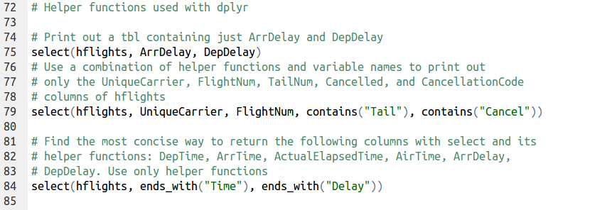
    # Use a combination of helper functions and variable names to print out
    # only the UniqueCarrier, FlightNum, TailNum, Cancelled, and CancellationCode
    # columns of hflights
    select(hflights, UniqueCarrier, FlightNum, contains("Tail"), contains("Cancel"))
    # Find the most concise way to return the following columns with select and its
    # helper functions: DepTime, ArrTime, ActualElapsedTime, AirTime, ArrDelay,
    # DepDelay. Use only helper functions
    select(hflights, ends_with("Time"), ends_with("Delay"))
    view raw verbs02.R hosted with ❤ by GitHub

    In order to appreciate the usefulness of dplyr, here are some comparisons between base R and dplyr

    # Some comparisons to basic R
    # both hflights and dplyr are available
    ex1r <- hflights[c("TaxiIn","TaxiOut","Distance")]
    ex1d <- select(hflights, TaxiIn, TaxiOut, Distance)
    ex2r <- hflights[c("Year","Month","DayOfWeek","DepTime","ArrTime")]
    ex2d <- select(hflights, Year:ArrTime, -DayofMonth)
    ex3r <- hflights[c("TailNum","TaxiIn","TaxiOut")]
    ex3d <- select(hflights, TailNum, contains("Taxi"))
    view raw comparisons01.R hosted with ❤ by GitHub

    mutate() is the second of the five data manipulation functions. mutate() creates new columns which are added to a copy of the dataset.

    # Add the new variable ActualGroundTime to a copy of hflights and save the result as g1.
    g1 <- mutate(hflights, ActualGroundTime = ActualElapsedTime AirTime)
    # Add the new variable GroundTime to a g1. Save the result as g2.
    g2 <- mutate(g1, GroundTime = TaxiIn + TaxiOut)
    # Add the new variable AverageSpeed to g2. Save the result as g3.
    g3 <- mutate(g2, AverageSpeed = Distance / AirTime * 60)
    # Print out g3
    g3
    view raw verbs03.r hosted with ❤ by GitHub

    So far we have added variables to hflights one at a time, but we can also use mutate() to add multiple variables at once.

    # Add a second variable loss_percent to the dataset: m1
    m1 <- mutate(hflights, loss = ArrDelay – DepDelay, loss_percent = ((ArrDelay – DepDelay)/DepDelay)*100)
    # mutate() allows you to use a new variable while creating a next variable in the same call
    # Copy and adapt the previous command to reduce redendancy: m2
    m2 <- mutate(hflights, loss = ArrDelay – DepDelay, loss_percent = (loss/DepDelay) * 100 )
    # Add the three variables as described in the third instruction: m3
    m3 <- mutate(hflights, TotalTaxi = TaxiIn + TaxiOut, ActualGroundTime = ActualElapsedTime – AirTime, Diff = TotalTaxi – ActualGroundTime)
    view raw verbs04.r hosted with ❤ by GitHub
  • Generating Permutation Matrices in Octave / Matlab

    Generating Permutation Matrices in Octave / Matlab

    I have been doing Gilbert Strang’s linear algebra assignments, some of which require you to write short scripts in MatLab, though I use GNU Octave (which is kind of like a free MatLab). I was trying out this problem:

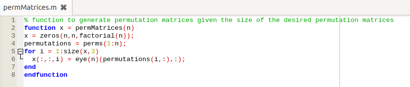
    permutationMatricesTo solve this quickly, it would have been nice to have a function that would give a list of permutation matrices for every n-sized square matrix, but there was none in Octave, so I wrote a function permMatrices which creates a list of permutation matrices for a square matrix of size n.
    % function to generate permutation matrices given the size of the desired permutation matrices
    function x = permMatrices(n)
    x = zeros(n,n,factorial(n));
    permutations = perms(1:n);
    for i = 1:size(x,3)
    x(:,:,i) = eye(n)(permutations(i,:),:);
    end
    endfunction
    view raw permMatrices.m hosted with ❤ by GitHub

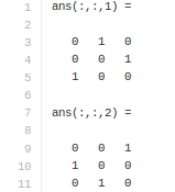
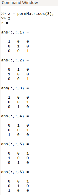
    For example:

    permMatrExample

    The MatLab / Octave code to solve this problem is shown below:

    % Solution for part (a)
    p = permMatrices(3);
    n = size(p,3); % number of permutation matrices
    v = zeros(n,1); % vector of zeros with dimension equalling number of permutation matrices
    % check for permutation matrices other than identity matrix with 3rd power equalling identity matrix
    for i = 1:n
    if p(:,:,i)^3 == eye(3)
    v(i,1) = 1;
    end
    end
    v(1,1) = 0; % exclude identity matrix
    ans1 = p(:,:,v == 1)
    % Solution for part (b)
    P = permMatrices(4);
    m = size(P,3); % number of permutation matrices
    t = zeros(m,1); % vector of zeros with dimension equalling number of permutation matrices
    % check for permutation matrices with 4th power equalling identity matrix
    for i = 1:m
    if P(:,:,i)^4 == eye(4)
    t(i,1) = 1;
    end
    end
    % print the permutation matrices
    ans2 = P(:,:,t == 0)
    view raw Section2_7_13.m hosted with ❤ by GitHub

    Output:

    op13a
    Output for 13(a)
    op13b
    Output for 13(b)


  • Sherlock and the Beast – HackerRank

    Sherlock and the Beast – HackerRank

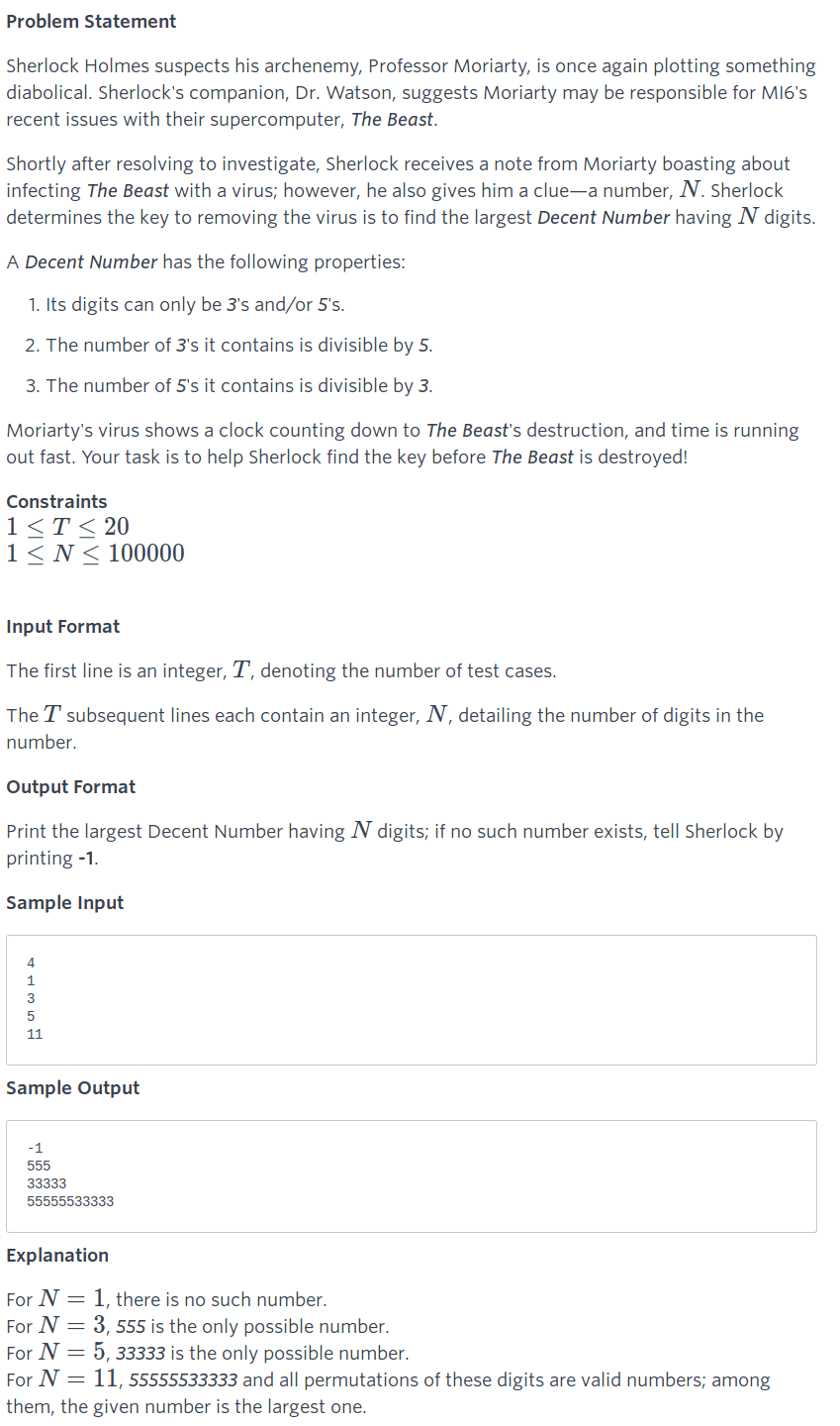
    I found myself stuck on this problem recently. I must confess, I lost a couple of hours trying to get to figure the logic for this one. Here’s the problem:

    sherlockAndTheBeast

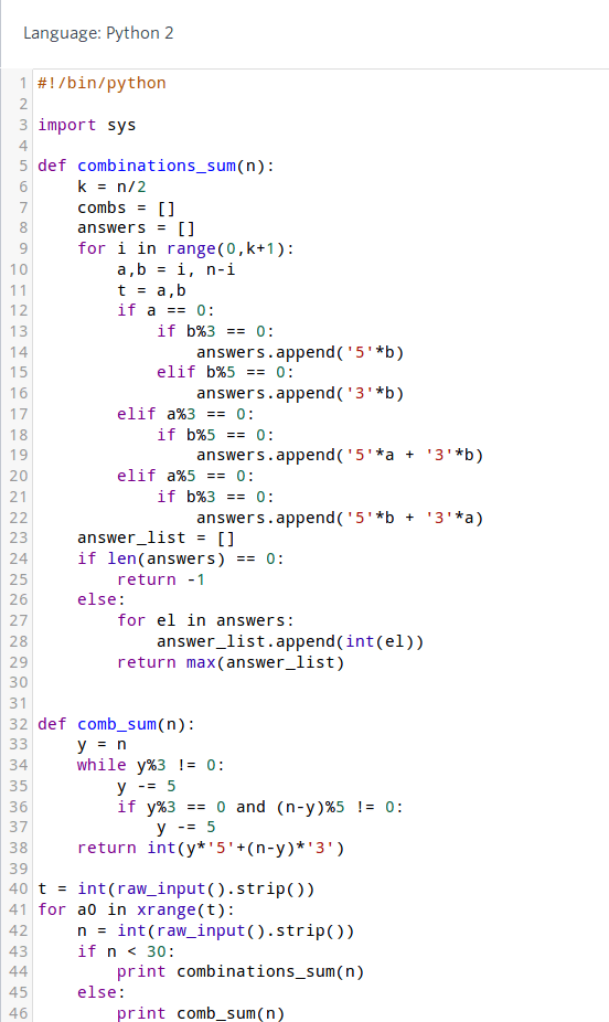
    I’ve written 2 functions to solve this problem. The first one I used for smaller N, say N < 30 and the second one for N > 30. The second function is elegant, and it relies on the mathematical property that if a number N is not divisible by 3, it could either leave a remainder 1 or 2.

    If it leaves a remainder 2, then subtracting 5 once would make the number divisible by 3. If it leaves a remainder 1, then subtracting 5 twice would make the number divisible by 3.

    We subtract 5 from N iteratively and attempt to divide N into 2 parts, one divisible by 3 and the other divisible by 5. We want the part that is divisible by 3 to be the larger part, so that the associated Decent Number is the largest possible. This explanation might seem obtuse, but if you get pen down on paper, you’ll understand what I mean.

    Solution

    sherlockAndTheBeastSol

  • Supplementary Material to Andrew Ng’s Machine Learning MOOC

    Supplementary Material to Andrew Ng’s Machine Learning MOOC

    Although the lecture videos and lecture notes from Andrew Ng‘s Coursera MOOC are sufficient for the online version of the course, if you’re interested in more mathematical stuff or want to be challenged further, you can go through the following notes and problem sets from CS 229, a 10-week course that he teaches at Stanford (which also happens to be the most enrolled course on campus). It’s not hard to end up with a 100% score on his MOOC which is obviously a (much) watered down version of the course he teaches at Stanford, at least in terms of difficulty. If you don’t believe me, just have a go at the problem sets from the links below.

    Lecture Notes

    Section Notes

    Handouts and Problem Sets

  • Solutions to Machine Learning Programming Assignments

    Solutions to Machine Learning Programming Assignments

    This post contains links to a bunch of code that I have written to complete Andrew Ng’s famous machine learning course which includes several interesting machine learning problems that needed to be solved using the Octave / Matlab programming language. I’m not sure I’d ever be programming in Octave after this course, but learning Octave just so that I could complete this course seemed worth the time and effort. I would usually work on the programming assignments on Sundays and spend several hours coding in Octave, telling myself that I would later replicate the exercises in Python.

    If you’ve taken this course and found some of the assignments hard to complete, I think it might not hurt to go check online on how a particular function was implemented. If you end up copying the entire code, it’s probably your loss in the long run. But then John Maynard Keynes once said, ‘In the long run we are all dead‘. Yeah, and we wonder why people call Economics the dismal science!

    Most people disregard Coursera’s feeble attempt at reigning in plagiarism by creating an Honor Code, precisely because this so-called code-of-conduct can be easily circumvented. I don’t mind posting solutions to a course’s programming assignments because GitHub is full to the brim with such content. Plus, it’s always good to read others’ code even if you implemented a function correctly. It helps understand the different ways of tackling a given programming problem.

    ex1
    ex2
    ex3
    ex4
    ex5
    ex6
    ex7
    ex8

    Enjoy!


  • Troubleshooting ‘Rattle’ (R library) Installation on Ubuntu

    Troubleshooting ‘Rattle’ (R library) Installation on Ubuntu

    This post pertains to Ubuntu / Debian users only.

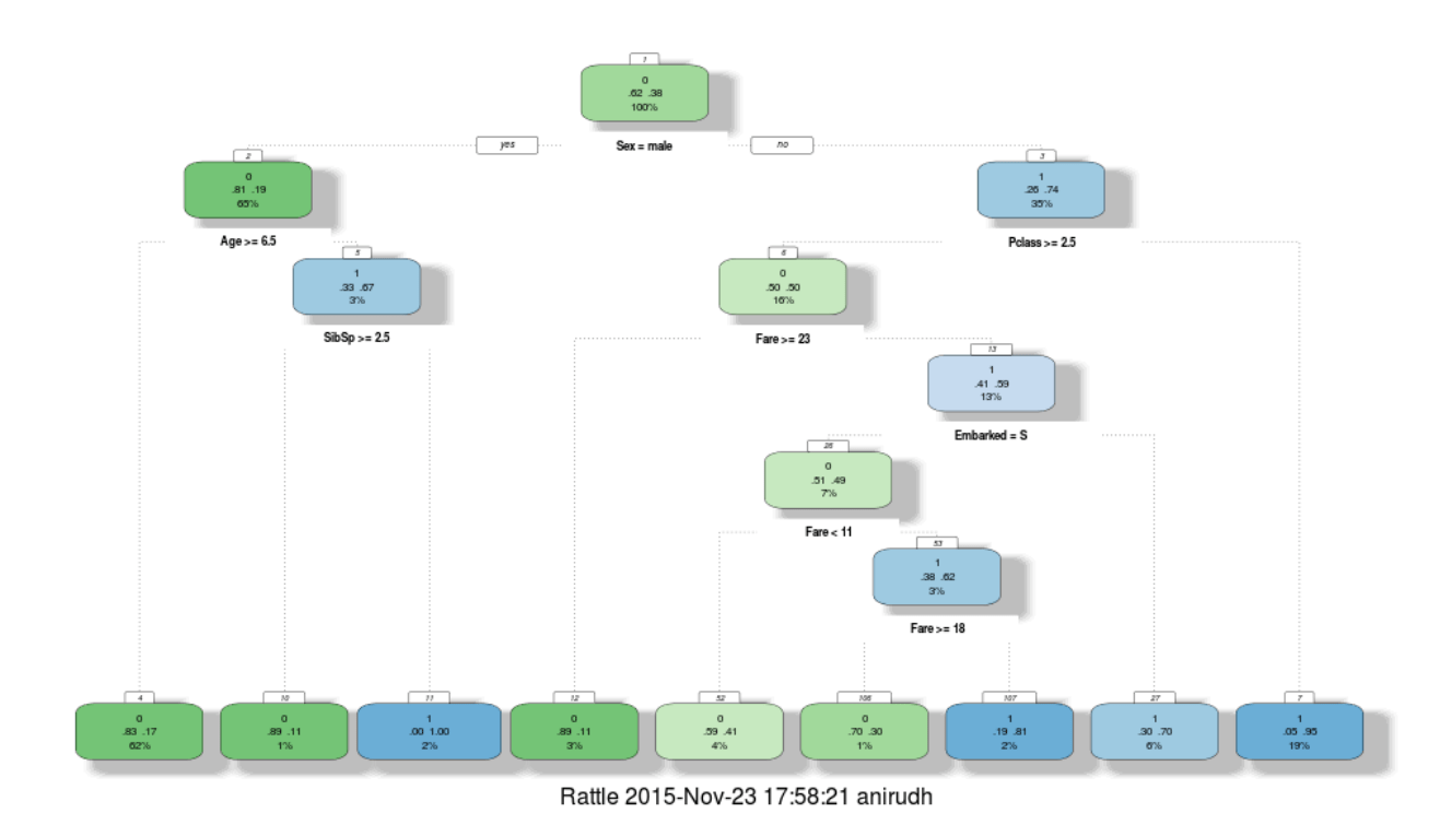
    rattle is a free graphical interface for data mining with R. I wanted to visualize decision trees and had to install this library.
    > install.packages('rattle')
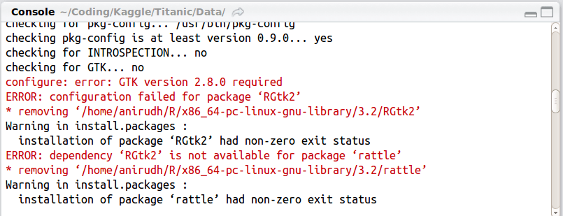
    got me the following error message:

    configure: error: GTK version 2.8.0 required
    ERROR: configuration failed for package ‘RGtk2’

    rattle_installationNonZeroExit

    This error occurs when attempting to install the RGtk2 package. The install is looking for the header files for GTK. Possibly they are not yet. Luckily the problem can be solved quite easily. Open Terminal (Ctrl + Alt + T) and type in the following commands:


    sudo apt-get update
    wajig install libgtk2.0-dev

    Go back and try installing rattle now with the same command as earlier. It should work. It did for me! As you can see below, decision trees are visualized lot better with rattle than if you used just rpart.

    rattle

  • Spot the Difference — It’s NumPy!

    Spot the Difference — It’s NumPy!

    My first brush with NumPy happened over writing a block of code to make a plot using pylab. ⇣


    pylab is part of matplotlib (in matplotlib.pylab) and tries to give you a MatLab like environment. matplotlib has a number of dependencies, among them numpy which it imports under the common alias np. scipy is not a dependency of matplotlib.


    I had a tuple (of lows and highs of temperature) of lengh 2 with 31 entries in each (the number of days in the month of July), parsed from this text file:

    Boston July Temperatures
    ————————-
    Day High Low
    ————
    1 91 70
    2 84 69
    3 86 68
    4 84 68
    5 83 70
    6 80 68
    7 86 73
    8 89 71
    9 84 67
    10 83 65
    11 80 66
    12 86 63
    13 90 69
    14 91 72
    15 91 72
    16 88 72
    17 97 76
    18 89 70
    19 74 66
    20 71 64
    21 74 61
    22 84 61
    23 86 66
    24 91 68
    25 83 65
    26 84 66
    27 79 64
    28 72 63
    29 73 64
    30 81 63
    31 73 63
    view raw julyTemps.txt hosted with ❤ by GitHub

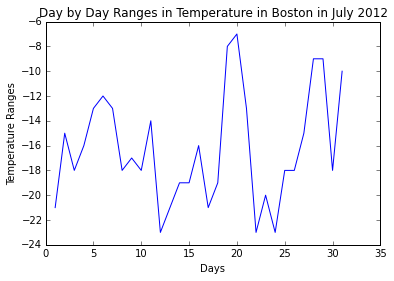
    Given below, are 2 sets of code that do the same thing; one without NumPy and the other with NumPy. They output the following graph using PyLab:

    differenceTemp

    Code without NumPy

    import pylab
    def loadfile():
    inFile = open('julyTemps.txt', 'r')
    high =[]; low = []
    for line in inFile:
    fields = line.split()
    if len(fields) < 3 or not fields[0].isdigit():
    pass
    else:
    high.append(int(fields[1]))
    low.append(int(fields[2]))
    return low, high
    def producePlot(lowTemps, highTemps):
    diffTemps = [highTemps[i] – lowTemps[i] for i in range(len(lowTemps))]
    pylab.title('Day by Day Ranges in Temperature in Boston in July 2012')
    pylab.xlabel('Days')
    pylab.ylabel('Temperature Ranges')
    return pylab.plot(range(1,32),diffTemps)
    producePlot(loadfile()[1], loadfile()[0])
    view raw withoutNumPy.py hosted with ❤ by GitHub

    Code with NumPy
    import pylab
    import numpy as np
    def loadFile():
    inFile = open('julyTemps.txt')
    high = [];vlow = []
    for line in inFile:
    fields = line.split()
    if len(fields) != 3 or 'Boston' == fields[0] or 'Day' == fields[0]:
    continue
    else:
    high.append(int(fields[1]))
    low.append(int(fields[2]))
    return (low, high)
    def producePlot(lowTemps, highTemps):
    diffTemps = list(np.array(highTemps) – np.array(lowTemps))
    pylab.plot(range(1,32), diffTemps)
    pylab.title('Day by Day Ranges in Temperature in Boston in July 2012')
    pylab.xlabel('Days')
    pylab.ylabel('Temperature Ranges')
    pylab.show()
    (low, high) = loadFile()
    producePlot(low, high)
    view raw withNumPy.py hosted with ❤ by GitHub

    The difference in code lies in how the variable diffTemps is calculated.

    diffTemps = list(np.array(highTemps) - np.array(lowTemps))
    

    seems more readable than

    diffTemps = [highTemps[i] - lowTemps[i] for i in range(len(lowTemps))]
    

    Notice how straight forward it is with NumPy. At the core of the NumPy package, is the ndarray object. This encapsulates n-dimensional arrays of homogeneous data types, with many operations being performed in compiled code for performance. element-by-element operations are the “default mode” when an ndarray is involved, but the element-by-element operation is speedily executed by pre-compiled C code.

  • Karatsuba Multiplication Algorithm – Python Code

    Karatsuba Multiplication Algorithm – Python Code

    Motivation for this blog post

    I’ve enrolled in Stanford Professor Tim Roughgarden’s Coursera MOOC on the design and analysis of algorithms, and while he covers the theory and intuition behind the algorithms in a surprising amount of detail, we’re left to implement them in a programming language of our choice.

    And I’m ging to post Python code for all the algorithms covered during the course!

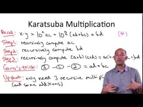
    The Karatsuba Multiplication Algorithm

    Karatsuba’s algorithm reduces the multiplication of two n-digit numbers to at most  n^{\log_23}\approx n^{1.585} single-digit multiplications in general (and exactly n^{\log_23} when n is a power of 2). Although the familiar grade school algorithm for multiplying numbers is how we work through multiplication in our day-to-day lives, it’s slower (\Theta(n^2)\,\!) in comparison, but only on a computer, of course!

    Here’s how the grade school algorithm looks:
    (The following slides have been taken from Tim Roughgarden’s notes. They serve as a good illustration. I hope he doesn’t mind my sharing them.)

    gradeSchoolAlgorithm

    …and this is how Karatsuba Multiplication works on the same problem:

    exampleKaratsuba

    recursiveKaratsuba

    A More General Treatment

    Let x and y be represented as n-digit strings in some base B. For any positive integer m less than n, one can write the two given numbers as

    x = x_1B^m + x_0
    y = y_1B^m + y_0,

    where x_0 and y_0 are less than B^m. The product is then

    xy = (x_1B^m + x_0)(y_1B^m + y_0)
    xy = z_2B^{2m} + z_1B^m + z_0

    where

    z_2 = x_1y_1
    z_1 = x_1y_0 + x_0y_1
    z_0 = x_0y_0

    These formulae require four multiplications, and were known to Charles Babbage. Karatsuba observed that xy can be computed in only three multiplications, at the cost of a few extra additions. With z_0 and z_2 as before we can calculate

    z_1 = (x_1 + x_0)(y_1 + y_0) - z_2 - z_0

    which holds since

    z_1 = x_1y_0 + x_0y_1
    z_1 = (x_1 + x_0)(y_1 + y_0) - x_1y_1 - x_0y_0

    A more efficient implementation of Karatsuba multiplication can be set as xy = (b^2 + b)x_1y_1 - b(x_1 - x_0)(y_1 - y_0) + (b + 1)x_0y_0, where b = B^m.

    Example

    To compute the product of 12345 and 6789, choose B = 10 and m = 3. Then we decompose the input operands using the resulting base (Bm = 1000), as:

    12345 = 12 · 1000 + 345
    6789 = 6 · 1000 + 789

    Only three multiplications, which operate on smaller integers, are used to compute three partial results:

    z2 = 12 × 6 = 72
    z0 = 345 × 789 = 272205
    z1 = (12 + 345) × (6 + 789) − z2z0 = 357 × 795 − 72 − 272205 = 283815 − 72 − 272205 = 11538

    We get the result by just adding these three partial results, shifted accordingly (and then taking carries into account by decomposing these three inputs in base 1000 like for the input operands):

    result = z2 · B2m + z1 · Bm + z0, i.e.
    result = 72 · 10002 + 11538 · 1000 + 272205 = 83810205.

    Pseudocode and Python code

    procedure karatsuba(num1, num2)
    if (num1 < 10) or (num2 < 10)
    return num1*num2
    /* calculates the size of the numbers */
    m = max(size_base10(num1), size_base10(num2))
    m2 = m/2
    /* split the digit sequences about the middle */
    high1, low1 = split_at(num1, m2)
    high2, low2 = split_at(num2, m2)
    /* 3 calls made to numbers approximately half the size */
    z0 = karatsuba(low1,low2)
    z1 = karatsuba((low1+high1),(low2+high2))
    z2 = karatsuba(high1,high2)
    return (z2*10^(2*m2))+((z1-z2-z0)*10^(m2))+(z0)

    def karatsuba(x,y):
    """Function to multiply 2 numbers in a more efficient manner than the grade school algorithm"""
    if len(str(x)) == 1 or len(str(y)) == 1:
    return x*y
    else:
    n = max(len(str(x)),len(str(y)))
    nby2 = n / 2
    a = x / 10**(nby2)
    b = x % 10**(nby2)
    c = y / 10**(nby2)
    d = y % 10**(nby2)
    ac = karatsuba(a,c)
    bd = karatsuba(b,d)
    ad_plus_bc = karatsuba(a+b,c+d) – ac – bd
    # this little trick, writing n as 2*nby2 takes care of both even and odd n
    prod = ac * 10**(2*nby2) + (ad_plus_bc * 10**nby2) + bd
    return prod
    view raw karatsuba.py hosted with ❤ by GitHub

  • Getting Started with R on MIT’s 14.74x (Foundations of Development Policy)

    Getting Started with R on MIT’s 14.74x (Foundations of Development Policy)

    I noticed that a major grievance of many students enrolled in MIT‘s latest edX course on development policy (Foundations of Development Policy: Advanced Development Economics) was that there wasn’t enough done to get them going with the R assignments. I have posted the R code for the homework (past the deadline, of course) of the first 2 weeks, so that others get a hang of the level of R that might be needed to solve these assignments in the following weeks. I’m willing to help out those needing help getting up to speed with R required for this course. For specific queries, leave your message in the comments section.

    A great place to get spend time learning R before taking Foundations of Development Policy (14.74x) would be another edX course that’s been getting great reviews recently: Introduction to R Programming

    R Code for Home Work (Week 1)

    # set working directory to local directory where the data is kept
    setwd("~/IGIDR/Development Economics – MIT/Homework Assignment 01")
    # read the data
    wb_dev_ind = read.csv("wb_dev_ind.csv")
    # summarize data
    summary(wb_dev_ind)
    # Question 1
    # What is the Mean of GDP per capita? What is the standard deviation of GDP per capita?
    meanGDPperCapita = mean(wb_dev_ind$gdp_per_capita, na.rm = TRUE)
    print(round(meanGDPperCapita))
    sdGDPperCapita = sd(wb_dev_ind$gdp_per_capita, na.rm = TRUE)
    print(round(sdGDPperCapita))
    # Question 2
    # What is the mean illiteracy rate across all countries? What is the standard deviation?
    illiteracy_all = numeric(nrow(wb_dev_ind))
    wb_dev_ind$illiteracy_all = illiteracy_all
    wb_dev_ind$illiteracy_all = 100 – wb_dev_ind$literacy_all
    meanIlliteracy = mean(wb_dev_ind$illiteracy_all, na.rm = TRUE)
    print(round(meanIlliteracy))
    sdIlliteracy = sd(wb_dev_ind$illiteracy_all, na.rm = TRUE)
    print(round(sdIlliteracy))
    # Question 3
    # What is the mean infant mortality rate across all countries? What is the standard deviation?
    meanInfantMortality = mean(wb_dev_ind$infant_mortality, na.rm = TRUE)
    print(round(meanInfantMortality))
    sdInfantMortality = sd(wb_dev_ind$infant_mortality, na.rm = TRUE)
    print(round(sdInfantMortality))
    # Question 4
    # What is the mean male illiteracy rate? What is the mean female illiteracy rate?
    illiteracy_male = numeric(nrow(wb_dev_ind))
    wb_dev_ind$illiteracy_male = illiteracy_male
    wb_dev_ind$illiteracy_male = 100 – wb_dev_ind$literacy_male
    meanIlliteracyMale = mean(wb_dev_ind$illiteracy_male, na.rm = TRUE)
    print(round(meanIlliteracyMale))
    sdIlliteracyMale = sd(wb_dev_ind$illiteracy_male, na.rm = TRUE)
    print(round(sdIlliteracyMale))
    illiteracy_female = numeric(nrow(wb_dev_ind))
    wb_dev_ind$illiteracy_female = illiteracy_female
    wb_dev_ind$illiteracy_female = 100 – wb_dev_ind$literacy_female
    meanIlliteracyFemale = mean(wb_dev_ind$illiteracy_female, na.rm = TRUE)
    print(round(meanIlliteracyFemale))
    sdIlliteracyFemale = sd(wb_dev_ind$illiteracy_female, na.rm = TRUE)
    print(round(sdIlliteracyFemale))
    # Question 5
    # What are the mean, minimum, and maximum illiteracy rate among the 50 richest countries
    richest50 = wb_dev_ind[order(wb_dev_ind$gdp_per_capita, decreasing = TRUE),][1:50,]
    summary(richest50)
    # Question 6
    # What are the mean, minimum, and maximum illiteracy rate among the 50 poorest countries?
    poorest50 = wb_dev_ind[order(wb_dev_ind$gdp_per_capita),][1:50,]
    summary(poorest50)
    # Question 7
    # What are the mean, minimum, and maximum infant mortality rate among the 50 richest countries?
    summary(richest50)
    # Question 8
    # What are the mean, minimum, and maximum infant mortality rate among the 50 poorest countries?
    summary(poorest50)
    # Question 9
    # What is the median GDP per capita?
    summary(wb_dev_ind)
    # Question 10-12
    # Regress the infant mortality rate on per capita GDP, and then answer questions 10-12
    model1 = lm(infant_mortality ~ gdp_per_capita, data = wb_dev_ind)
    summary(model1)
    # Question 13
    # Regress the illiteracy rate on GDP per capita. Is the coefficient on per capita GDP significantly different from zero at the 5% level?
    model2 = lm(illiteracy_all ~ gdp_per_capita, data = wb_dev_ind)
    summary(model2)
    # Question 14
    # Regress the infant mortality rate on the illiteracy rate. Graph a scatter plot of the data as well as the regression line.
    model3 = lm(infant_mortality ~ illiteracy_all, data = wb_dev_ind)
    summary(model3)
    plot(wb_dev_ind$illiteracy_all, wb_dev_ind$infant_mortality)
    abline(model3)
    view raw HW01.R hosted with ❤ by GitHub

    R Code for Home Work (Week 2)

    # Set working directory to local directory where the data is kept
    setwd("~/IGIDR/Development Economics – MIT/Homework Assignment 02")
    # read data
    migueldata = read.csv("ted_miguel_worms.csv", header = TRUE)
    attach(migueldata)
    # Question 6
    # How many observations are there per pupil? (Enter a whole number of 0 or higher)?
    length(migueldata$pupid)
    length(unique(migueldata$pupid))
    # Question 7
    # What percentage of the pupils are boys? (Answers within 0.50 percentage points of the correct answer will be accepted. For instance, 67 would be accepted if the correct answer is 67.45%)
    mean(sex, na.rm = TRUE)
    # Question 8
    # What percentage of pupils took the deworming pill in 1998? (Answers within 0.50 percentage points of the correct answer will be accepted. For instance, 67 would be accepted if the correct answer is 67.45%)
    mean(pill98, na.rm = TRUE)
    # Question 9
    # Was the percentage of schools assigned to treatment in 1998 greater than or less than the percentage of pupils that actually took the deworming pill in 1998?
    mean(treat_sch98, na.rm = TRUE)
    mean(treat_sch98, na.rm = TRUE) > mean(pill98, na.rm = TRUE) # Ans = Greater Than
    # Question 10
    # Which of the following variables from the dataset are dummy variables? (Check all that apply.)
    summary(migueldata)
    # Question 11
    # Using the data, find and enter the difference in outcomes (Y: school participation) between students who took the pill and students who did not in 1998. (Enter your answer as a difference in proportions. For instance, if the proportion in one group is 0.61 and the proportion in the other group is 0.54, enter 0.07. Answers within 0.05 of the correct answer will be accepted. For instance, 0.28 would be accepted if the correct answer is 0.33.)
    took_pill_98 = mean(migueldata[migueldata$pill98 == 1,]$totpar98, na.rm = TRUE)
    no_pill_98 = mean(migueldata[migueldata$pill98 == 0,]$totpar98, na.rm = TRUE)
    diff = took_pill_98 – no_pill_98
    diff
    # Question 12
    # Since schools were randomly assigned to the deworming treatment group, the estimate calculated in the previous answer is an unbiased estimate of taking the pill on school attendance.
    # False
    # Explanation
    # The estimated impact of 13 percentage points calculated in the previous answer might not be a good estimate of the effect of taking the pill. Many students in the randomly assigned treatment schools did not actually take the pills, so those who took the pills would not have been randomly selected at all. For instance, kids who attend school more anyway might have been more likely to be there when the pills were handed out, meaning that omitted variables would be correlated with taking the pill and future school attendance. This would bias the estimate upward i.e. the 13 percentage point difference might overstate the impact of deworming on attendance.
    # Question 13
    # Using the data, find and enter the difference in outcomes (Y: school participation) between students in treatment schools and students not in treatment schools in 1998, regardless of whether or not they actually took the pill. (Enter your answer as a difference in proportions. For instance, if the proportion in one group is 0.61 and the proportion in the other group is 0.54, enter 0.07. Answers within 0.05 of the correct answer will be accepted. For instance, 0.28 would be accepted if the correct answer is 0.33.)
    in_treatment_sch = mean(migueldata[migueldata$treat_sch98 == 1,]$totpar98, na.rm = TRUE)
    non_treatment_sch = mean(migueldata[migueldata$treat_sch98 == 0,]$totpar98, na.rm = TRUE)
    diff_treatment_sch = in_treatment_sch – non_treatment_sch
    diff_treatment_sch
    # Question 14
    # Using the data, calculate the difference in the probability of taking the pill given that a student was in a treatment school and the probability of taking it if a student was not in a treatment school. (Enter your answer as a difference in proportions. For instance, if the proportion in one group is 0.61 and the proportion in the other group is 0.54, enter 0.07. Answers within 0.05 of the correct answer will be accepted. For instance, 0.28 would be accepted if the correct answer is 0.33.)
    pr_pill_treatment_sch = mean(migueldata[migueldata$treat_sch98 == 1,]$pill98, na.rm = TRUE)
    pr_pill_no_treatment_sch = mean(migueldata[migueldata$treat_sch98 == 0,]$pill98, na.rm = TRUE)
    diff_pr_pill_treatment_sch = pr_pill_treatment_sch – pr_pill_no_treatment_sch
    # Question 15
    # Using the data, derive the Wald Estimator of taking the pill on school attendance. (Enter your answer as a difference in proportions. For instance, if the proportion in one group is 0.61 and the proportion in the other group is 0.54, enter 0.07. Answers within 0.05 of the correct answer will be accepted. For instance, 0.28 would be accepted if the correct answer is 0.33.)
    waldRatio = diff_treatment_sch/diff_pr_pill_treatment_sch
    waldRatio
    view raw HW02.R hosted with ❤ by GitHub

    I hope this helps!

  • Scatter Plot Bug Fix in Dato’s GraphLab Create ML Package in Python

    Scatter Plot Bug Fix in Dato’s GraphLab Create ML Package in Python

    I have been using Dato’s GraphLab Create for Coursera’s new Machine Learning Specialization that uses Python. Like me, if you’ve been facing trouble obtaining scatter plots on your canvas in GraphLab Create despite the following code:

    graphlab.canvas.set_target('ipynb')

    …then no worries, there is a quick fix. I’ve been deliberately lousy with the presentation, so sorry about that. Chances are that no one’s going to end up reading this anyway. I saw this problem being discussed on a Dato forum, so I decided to blog about the fix.

    EDIT: Note that this problem is in GraphLab Create v1.6 only. They came up with v1.6.1 a few days after the problem was escalated on their forum, so a good option would be to upgrade GraphLab Create.

    The problem you face should looks something like this (click images below to enlarge):Screenshot from 2015-09-25 14:10:20

    To solve the problem:

    Locate sframe.py from your home directory by searching for it from your desktop environment (applies to Windows users too). I found it in the following path on my computer:

    ~/anaconda/lib/python2.7/site-packages/graphlab/canvas/views

    The file sframe.py should look like this:

    Screenshot from 2015-09-25 15:49:44

    Then replace the code in lines 255-227 of the opened .py file with the code highlighted below:

    Screenshot from 2015-09-25 15:53:19

    This should take care of the problem for good.

    Now you have your desired result:

    Screenshot from 2015-09-25 16:18:41