Through this post, I’m sharing Python code implementing the median of medians algorithm, an algorithm that resembles quickselect, differing only in the way in which the pivot is chosen, i.e, deterministically, instead of at random.
Its best case complexity is O(n) and worst case complexity O(nlog2n)
I don’t have a formal education in CS, and came across this algorithm while going through Tim Roughgarden’s Coursera MOOC on the design and analysis of algorithms. Check out my implementation in Python.
This file contains hidden or bidirectional Unicode text that may be interpreted or compiled differently than what appears below. To review, open the file in an editor that reveals hidden Unicode characters.
Learn more about bidirectional Unicode characters
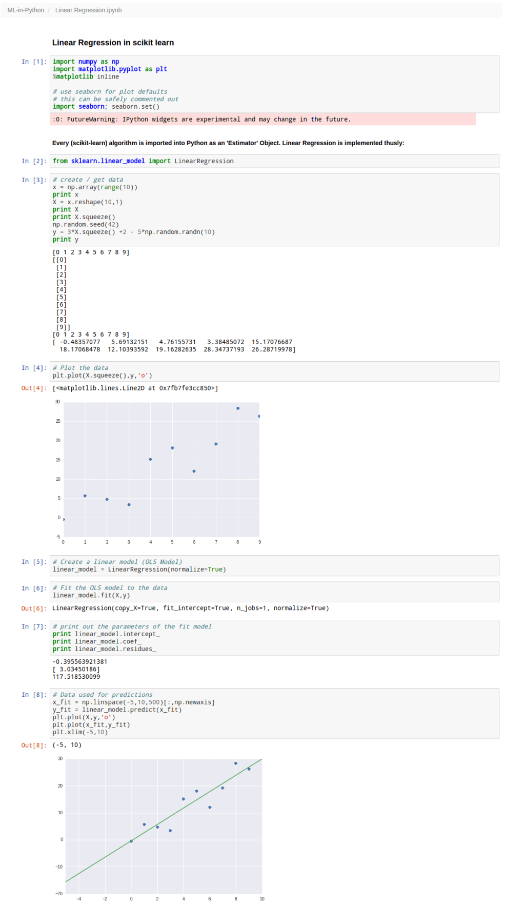
Here’s a quick example case for implementing one of the simplest of learning algorithms in any machine learning toolbox – Linear Regression. You can download the IPython / Jupyter notebook here so as to play around with the code and try things out yourself.
I’m doing a series of posts on scikit-learn. Its documentation is vast, so unless you’re willing to search for a needle in a haystack, you’re better off NOT jumping into the documentation right away. Instead, knowing chunks of code that do the job might help.
Find the kth smallest element in an array without sorting.
That’s basically what this algorithm does. It piggybacks on the partition subroutine from the Quick Sort. If you don’t know what that is, you can check out more about the Quick Sort algorithm here and here, and understand the usefulness of partitioning an unsorted array around a pivot.
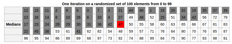
Animated visualization of the randomized selection algorithm selecting the 22nd smallest value
Python Implementation
This file contains hidden or bidirectional Unicode text that may be interpreted or compiled differently than what appears below. To review, open the file in an editor that reveals hidden Unicode characters.
Learn more about bidirectional Unicode characters
A key aspect of the Quick Sort algorithm is how the pivot element is chosen. In my earlier post on the Python code for Quick Sort, my implementation takes the first element of the unsorted array as the pivot element.
However with some mathematical analysis it can be seen that such an implementation is O(n2) in complexity while if a pivot is randomly chosen, the Quick Sort algorithm is O(nlog2n).
To witness this in action, one can measure the work done by the algorithm comparing two cases, one with a randomized pivot choice – and one with a fixed pivot choice, say the first element of the array (or the last element of the array).
Implementation
A decent proxy for the amount of work done by the algorithm would be the number of pivot comparisons. These comparisons needn’t be computed one-by-one, rather when there is a recursive call on a subarray of length m, you should simply add m−1 to your running total of comparisons.
3 Cases
To put things in perspective, let’s look at 3 cases. (This is basically straight out of a homework assignment from Tim Roughgarden’s course on the Design and Analysis of Algorithms). Case I with the pivot being the first element. Case II with the pivot being the last element. Case III using the “median-of-three” pivot rule. The primary motivation behind this rule is to do a little bit of extra work to get much better performance on input arrays that are nearly sorted or reverse sorted.
Median-of-Three Pivot Rule
Consider the first, middle, and final elements of the given array. (If the array has odd length it should be clear what the “middle” element is; for an array with even length 2k, use the kth element as the “middle” element. So for the array 4 5 6 7, the “middle” element is the second one —- 5 and not 6! Identify which of these three elements is the median (i.e., the one whose value is in between the other two), and use this as your pivot.
This file contains all of the integers between 1 and 10,000 (inclusive, with no repeats) in unsorted order. The integer in the ith row of the file gives you the ith entry of an input array. I downloaded this file and named it QuickSort_List.txt
You can run the code below and see for yourself that the number of comparisons for Case III are 138,382 compared to 162,085 and 164,123 for Case I and Case II respectively. You can play around with the code in an IPython / Jupyter notebook here.
This file contains hidden or bidirectional Unicode text that may be interpreted or compiled differently than what appears below. To review, open the file in an editor that reveals hidden Unicode characters.
Learn more about bidirectional Unicode characters
Yet another post for the crawlers to better index my site for algorithms and as a repository for Python code. The quick sort algorithm is well explained in the topmost Google search result for ‘Quick Sort Python Code’, but the code is unnecessarily convoluted. Instead, go with the code below.
In it, I assume the pivot to be the first element. You can easily add a function to randomize selection of the pivot. Choosing a random pivot minimizes the chance that you will encounter worst-case O(n2) performance. Always choosing first or last would cause worst-case performance for nearly-sorted or nearly-reverse-sorted data.
This file contains hidden or bidirectional Unicode text that may be interpreted or compiled differently than what appears below. To review, open the file in an editor that reveals hidden Unicode characters.
Learn more about bidirectional Unicode characters
Edit: This post is in its infancy. Work is still ongoing as far as deriving insight from the data is concerned. More content and economic insight is expected to be added to this post as and when progress is made in that direction.
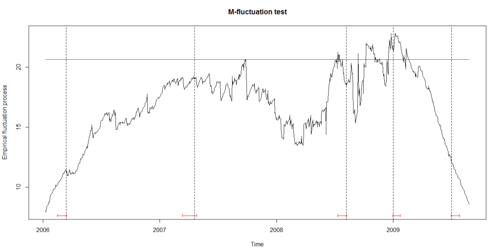
This is an attempt to detect structural breaks in China’s FX regime using Frenkel Wei regression methodology (this was later improved by Perron and Bai). I came up with the motivation to check for these structural breaks while attending a guest lecture on FX regimes by Dr. Ajay Shah delivered at IGIDR. This is work that I and two other classmates are working on as a term paper project under the supervision of Dr. Rajeswari Sengupta.
The code below can be replicated and run as is, to get same results.
This file contains hidden or bidirectional Unicode text that may be interpreted or compiled differently than what appears below. To review, open the file in an editor that reveals hidden Unicode characters.
Learn more about bidirectional Unicode characters
As can be seen in the figure below, the structural breaks correspond to the vertical bars. We are still working on understanding the motivations of China’s central bank in varying the degree of the managed float exchange rate.
EDIT (May 16, 2016):
The code above uses data provided by the package itself. If you wished to replicate this analysis on data after 2010, you will have to use your own data. We used Quandl, which lets you get 10 premium datasets for free. An API key (for only 10 calls on premium datasets) is provided if you register there. Foreign exchange rate data (2000 onward till date) apparently, is premium data. You can find these here.
Here are the (partial) results and code to work the same methodology on the data from 2010 to 2016:
This file contains hidden or bidirectional Unicode text that may be interpreted or compiled differently than what appears below. To review, open the file in an editor that reveals hidden Unicode characters.
Learn more about bidirectional Unicode characters
We got breaks in 2010 and in 2015 (when China’s stock markets crashed). We would have hoped for more breaks (we can still get them), but that would depend on the parameters chosen for our regression.
Deep learning became a hot topic in machine learning in the last 3-4 years (see inset below) and recently, Google released TensorFlow (a Python based deep learning toolkit) as an open source project to bring deep learning to everyone.
Interest in the Google search term Deep Learning over time
If you have wanted to get your hands dirty with TensorFlow or needed more direction with that, here’s some good news – Google is offering an open MOOC on deep learning methods using TensorFlow here. This course has been developed with Vincent Vanhoucke, Principal Scientist at Google, and technical lead in the Google Brain team. However, this is an intermediate to advanced level course and assumes you have taken a first course in machine learning, or that you are at least familiar with supervised learning methods.
Google’s overall goal in designing this course is to provide the machine learning enthusiast a rapid and direct path to solving real and interesting problems with deep learning techniques.
This happens to be my 50th blog post – and my blog is 8 months old.
🙂
This post is the third and last post in in a series of posts (Part 1 – Part 2) on data manipulation with dlpyr. Note that the objects in the code may have been defined in earlier posts and the code in this post is in continuation with code from the earlier posts.
Although datasets can be manipulated in sophisticated ways by linking the 5 verbs of dplyr in conjunction, linking verbs together can be a bit verbose.
Creating multiple objects, especially when working on a large dataset can slow you down in your analysis. Chaining functions directly together into one line of code is difficult to read. This is sometimes called the Dagwood sandwich problem: you have too much filling (too many long arguments) between your slices of bread (parentheses). Functions and arguments get further and further apart.
The %>% operator allows you to extract the first argument of a function from the arguments list and put it in front of it, thus solving the Dagwood sandwich problem.
This file contains hidden or bidirectional Unicode text that may be interpreted or compiled differently than what appears below. To review, open the file in an editor that reveals hidden Unicode characters.
Learn more about bidirectional Unicode characters
group_by() defines groups within a data set. Its influence becomes clear when calling summarise() on a grouped dataset. Summarizing statistics are calculated for the different groups separately.
This file contains hidden or bidirectional Unicode text that may be interpreted or compiled differently than what appears below. To review, open the file in an editor that reveals hidden Unicode characters.
Learn more about bidirectional Unicode characters
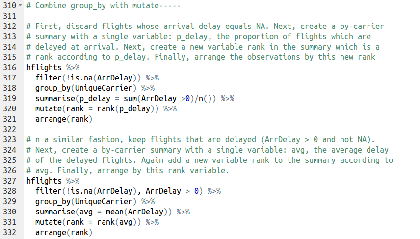
group_by() can also be combined with mutate(). When you mutate grouped data, mutate() will calculate the new variables independently for each group. This is particularly useful when mutate() uses the rank() function, that calculates within group rankings. rank() takes a group of values and calculates the rank of each value within the group, e.g.
rank(c(21, 22, 24, 23))
has output
[1] 1 2 4 3
As with arrange(), rank() ranks values from the largest to the smallest and this behaviour can be reversed with the desc() function.
This file contains hidden or bidirectional Unicode text that may be interpreted or compiled differently than what appears below. To review, open the file in an editor that reveals hidden Unicode characters.
Learn more about bidirectional Unicode characters
Note that this post is in continuation with Part 1 of this series of posts on data manipulation with dplyr in R. The code in this post carries forward from the variables / objects defined in Part 1.
In the previous post, I talked about how dplyr provides a grammar of sorts to manipulate data, and consists of 5 verbs to do so:
The 5 verbs of dplyr select – removes columns from a dataset filter – removes rows from a dataset arrange – reorders rows in a dataset mutate – uses the data to build new columns and values summarize – calculates summary statistics
I went on to discuss examples using select() and mutate(). Let’s now talk about filter(). R comes with a set of logical operators that you can use inside filter(). These operators are: x < y,TRUE if x is less than y x <= y, TRUE if x is less than or equal to y x == y, TRUE if x equals y x != y, TRUE if x does not equal y x >= y, TRUE if x is greater than or equal to y x > y, TRUE if x is greater than y x %in% c(a, b, c), TRUE if x is in the vector c(a, b, c)
The following call, for example, filters df such that only the observations where the variable a is greater than the variable b: filter(df, a > b)
This file contains hidden or bidirectional Unicode text that may be interpreted or compiled differently than what appears below. To review, open the file in an editor that reveals hidden Unicode characters.
Learn more about bidirectional Unicode characters
Combining tests using boolean operators
R also comes with a set of boolean operators that you can use to combine multiple logical tests into a single test. These include & (and), | (or), and ! (not). Instead of using the & operator, you can also pass several logical tests to filter(), separated by commas. The following calls equivalent:
filter(df, a > b & c > d) filter(df, a > b, c > d)
The is.na() will also come in handy very often. This expression, for example, keeps the observations in df for which the variable x is not NA:
filter(df, !is.na(x))
This file contains hidden or bidirectional Unicode text that may be interpreted or compiled differently than what appears below. To review, open the file in an editor that reveals hidden Unicode characters.
Learn more about bidirectional Unicode characters
This file contains hidden or bidirectional Unicode text that may be interpreted or compiled differently than what appears below. To review, open the file in an editor that reveals hidden Unicode characters.
Learn more about bidirectional Unicode characters
Arranging Data arrange() can be used to rearrange rows according to any type of data. If you pass arrange() a character variable, R will rearrange the rows in alphabetical order according to values of the variable. If you pass a factor variable, R will rearrange the rows according to the order of the levels in your factor (running levels() on the variable reveals this order).
By default, arrange() arranges the rows from smallest to largest. Rows with the smallest value of the variable will appear at the top of the data set. You can reverse this behaviour with the desc() function. arrange() will reorder the rows from largest to smallest values of a variable if you wrap the variable name in desc() before passing it to arrange()
This file contains hidden or bidirectional Unicode text that may be interpreted or compiled differently than what appears below. To review, open the file in an editor that reveals hidden Unicode characters.
Learn more about bidirectional Unicode characters
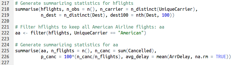
summarise(), the last of the 5 verbs, follows the same syntax as mutate(), but the resulting dataset consists of a single row instead of an entire new column in the case of mutate().
In contrast to the four other data manipulation functions, summarise() does not return an altered copy of the dataset it is summarizing; instead, it builds a new dataset that contains only the summarizing statistics.
Note:summarise() and summarize() both work the same!
You can use any function you like in summarise(), so long as the function can take a vector of data and return a single number. R contains many aggregating functions. Here are some of the most useful:
min(x) – minimum value of vector x. max(x) – maximum value of vector x. mean(x) – mean value of vector x. median(x) – median value of vector x. quantile(x, p) – pth quantile of vector x. sd(x) – standard deviation of vector x. var(x) – variance of vector x. IQR(x) – Inter Quartile Range (IQR) of vector x. diff(range(x)) – total range of vector x.
This file contains hidden or bidirectional Unicode text that may be interpreted or compiled differently than what appears below. To review, open the file in an editor that reveals hidden Unicode characters.
Learn more about bidirectional Unicode characters
dplyr provides several helpful aggregate functions of its own, in addition to the ones that are already defined in R. These include:
first(x) – The first element of vector x. last(x) – The last element of vector x. nth(x, n) – The nth element of vector x. n() – The number of rows in the data.frame or group of observations that summarise() describes. n_distinct(x) – The number of unique values in vector x
This file contains hidden or bidirectional Unicode text that may be interpreted or compiled differently than what appears below. To review, open the file in an editor that reveals hidden Unicode characters.
Learn more about bidirectional Unicode characters
This would be it for Part-2 of this series of posts on data manipulation with dplyr. Part 3 would focus on the pipe operator, Group_by and working with databases.