dplyr is one of the packages in R that makes R so loved by data scientists. It has three main goals:
- Identify the most important data manipulation tools needed for data analysis and make them easy to use in R.
- Provide blazing fast performance for in-memory data by writing key pieces of code in C++.
- Use the same code interface to work with data no matter where it’s stored, whether in a data frame, a data table or database.
Introduction to the dplyr package and the tbl class
This post is mostly about code. If you’re interested in learning dplyr I recommend you type in the commands line by line on the R console to see first hand what’s happening.
| # INTRODUCTION TO dplyr AND tbls | |
| # Load the dplyr package | |
| library(dplyr) | |
| # Load the hflights package | |
| library(hflights) | |
| # Call both head() and summary() on hflights | |
| head(hflights) | |
| summary(hflights) | |
| # Convert the hflights data.frame into a hflights tbl | |
| hflights <- tbl_df(hflights) | |
| # Display the hflights tbl | |
| hflights | |
| # Create the object carriers, containing only the UniqueCarrier variable of hflights | |
| carriers <- hflights$UniqueCarrier | |
| # Use lut to translate the UniqueCarrier column of hflights and before doing so | |
| # glimpse hflights to see the UniqueCarrier variablle | |
| glimpse(hflights) | |
| lut <- c("AA" = "American", "AS" = "Alaska", "B6" = "JetBlue", "CO" = "Continental", | |
| "DL" = "Delta", "OO" = "SkyWest", "UA" = "United", "US" = "US_Airways", | |
| "WN" = "Southwest", "EV" = "Atlantic_Southeast", "F9" = "Frontier", | |
| "FL" = "AirTran", "MQ" = "American_Eagle", "XE" = "ExpressJet", "YV" = "Mesa") | |
| hflights$UniqueCarrier <- lut[hflights$UniqueCarrier] | |
| # Now glimpse hflights to see the change in the UniqueCarrier variable | |
| glimpse(hflights) | |
| # Fill up empty entries of CancellationCode with 'E' | |
| # To do so, first index the empty entries in CancellationCode | |
| cancellationEmpty <- hflights$CancellationCode == "" | |
| # Assign 'E' to the empty entries | |
| hflights$CancellationCode[cancellationEmpty] <- 'E' | |
| # Use a new lookup table to create a vector of code labels. Assign the vector to the CancellationCode column of hflights | |
| lut = c('A' = 'carrier', 'B' = 'weather', 'C' = 'FFA', 'D' = 'security', 'E' = 'not cancelled') | |
| hflights$CancellationCode <- lut[hflights$CancellationCode] | |
| # Inspect the resulting raw values of your variables | |
| glimpse(hflights) |
Select and mutate
dplyr provides grammar for data manipulation apart from providing data structure. The grammar is built around 5 functions (also referred to as verbs) that do the basic tasks of data manipulation.
The 5 verbs of dplyr
select – removes columns from a dataset
filter – removes rows from a dataset
arrange – reorders rows in a dataset
mutate – uses the data to build new columns and values
summarize – calculates summary statistics
dplyr functions do not change the dataset. They return a new copy of the dataset to use.
To answer the simple question whether flight delays tend to shrink or grow during a flight, we can safely discard a lot of the variables of each flight. To select only the ones that matter, we can use select()
| hflights[c('ActualElapsedTime','ArrDelay','DepDelay')] | |
| # Equivalently, using dplyr: | |
| select(hflights, ActualElapsedTime, ArrDelay, DepDelay) | |
| # Print out a tbl with the four columns of hflights related to delay | |
| select(hflights, ActualElapsedTime, AirTime, ArrDelay, DepDelay) | |
| # Print out hflights, nothing has changed! | |
| hflights | |
| # Print out the columns Origin up to Cancelled of hflights | |
| select(hflights, Origin:Cancelled) | |
| # Find the most concise way to select: columns Year up to and | |
| # including DayOfWeek, columns ArrDelay up to and including Diverted | |
| # Answer to last question: be concise! | |
| # You may want to examine the order of hflight's column names before you | |
| # begin with names() | |
| names(hflights) | |
| select(hflights, -(DepTime:AirTime)) |
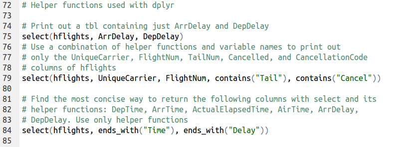
dplyr comes with a set of helper functions that can help you select variables. These functions find groups of variables to select, based on their names. Each of these works only when used inside of select()
- starts_with(“X”): every name that starts with “X”
- ends_with(“X”): every name that ends with “X”
- contains(“X”): every name that contains “X”
- matches(“X”): every name that matches “X”, where “X” can be a regular expression
- num_range(“x”, 1:5): the variables named x01, x02, x03, x04 and x05
- one_of(x): every name that appears in x, which should be a character vector
| # Helper functions used with dplyr | |
| # Print out a tbl containing just ArrDelay and DepDelay | |
| select(hflights, ArrDelay, DepDelay) | |
| # Use a combination of helper functions and variable names to print out | |
| # only the UniqueCarrier, FlightNum, TailNum, Cancelled, and CancellationCode | |
| # columns of hflights | |
| select(hflights, UniqueCarrier, FlightNum, contains("Tail"), contains("Cancel")) | |
| # Find the most concise way to return the following columns with select and its | |
| # helper functions: DepTime, ArrTime, ActualElapsedTime, AirTime, ArrDelay, | |
| # DepDelay. Use only helper functions | |
| select(hflights, ends_with("Time"), ends_with("Delay")) |
In order to appreciate the usefulness of dplyr, here are some comparisons between base R and dplyr
| # Some comparisons to basic R | |
| # both hflights and dplyr are available | |
| ex1r <- hflights[c("TaxiIn","TaxiOut","Distance")] | |
| ex1d <- select(hflights, TaxiIn, TaxiOut, Distance) | |
| ex2r <- hflights[c("Year","Month","DayOfWeek","DepTime","ArrTime")] | |
| ex2d <- select(hflights, Year:ArrTime, -DayofMonth) | |
| ex3r <- hflights[c("TailNum","TaxiIn","TaxiOut")] | |
| ex3d <- select(hflights, TailNum, contains("Taxi")) |
mutate() is the second of the five data manipulation functions. mutate() creates new columns which are added to a copy of the dataset.
| # Add the new variable ActualGroundTime to a copy of hflights and save the result as g1. | |
| g1 <- mutate(hflights, ActualGroundTime = ActualElapsedTime – AirTime) | |
| # Add the new variable GroundTime to a g1. Save the result as g2. | |
| g2 <- mutate(g1, GroundTime = TaxiIn + TaxiOut) | |
| # Add the new variable AverageSpeed to g2. Save the result as g3. | |
| g3 <- mutate(g2, AverageSpeed = Distance / AirTime * 60) | |
| # Print out g3 | |
| g3 |
So far we have added variables to hflights one at a time, but we can also use mutate() to add multiple variables at once.
| # Add a second variable loss_percent to the dataset: m1 | |
| m1 <- mutate(hflights, loss = ArrDelay – DepDelay, loss_percent = ((ArrDelay – DepDelay)/DepDelay)*100) | |
| # mutate() allows you to use a new variable while creating a next variable in the same call | |
| # Copy and adapt the previous command to reduce redendancy: m2 | |
| m2 <- mutate(hflights, loss = ArrDelay – DepDelay, loss_percent = (loss/DepDelay) * 100 ) | |
| # Add the three variables as described in the third instruction: m3 | |
| m3 <- mutate(hflights, TotalTaxi = TaxiIn + TaxiOut, ActualGroundTime = ActualElapsedTime – AirTime, Diff = TotalTaxi – ActualGroundTime) |
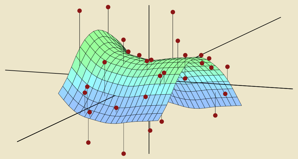


![Solution to [Viral] Math Puzzle for Vietnamese Eight-Year-Olds (Using R)](https://pythonandr.com/wp-content/uploads/2015/05/f7e7f4a5-b59c-4580-88f4-ddc609584d19-bestsizeavailable.png?w=497)