Quick Sort Python Code

July 8, 2016July 14, 2016 Anirudh Technical Algorithms, Python, Quick Sort, Sorting

Yet another post for the crawlers to better index my site for algorithms and as a repository for Python code. The quick sort algorithm is well explained in the topmost Google search result for ‘Quick Sort Python Code’, but the code is unnecessarily convoluted. Instead, go with the code below.

In it, I assume the pivot to be the first element. You can easily add a function to randomize selection of the pivot. Choosing a random pivot minimizes the chance that you will encounter worst-case O(n²) performance. Always choosing first or last would cause worst-case performance for nearly-sorted or nearly-reverse-sorted data.

	def quicksort(x):
	if len(x) == 1 or len(x) == 0:
	return x
	else:
	pivot = x[0]
	i = 0
	for j in range(len(x)-1):
	if x[j+1] < pivot:
	x[j+1],x[i+1] = x[i+1], x[j+1]
	i += 1
	x[0],x[i] = x[i],x[0]
	first_part = quicksort(x[:i])
	second_part = quicksort(x[i+1:])
	first_part.append(x[i])
	return first_part + second_part

	alist = [54,26,93,17,77,31,44,55,20]
	quicksort(alist)
	print(alist)

view raw quicksort.py hosted with ❤ by GitHub

Also read:
Computing Work Done (Total Pivot Comparisons) by Quick Sort
Karatsuba Multiplication Algorithm – Python Code
Merge Sort

How to become a Data Scientist in 6 months

June 15, 2016June 17, 2016 Anirudh Non Technical Data Science, Kaggle, Machine Learning, PyData, Python

Disclaimer: I’m not a data scientist yet. That’s still work in progress, but I’d recommend this excellent talk given by Tetiana Ivanova to put an enthusiast’s data science journey in perspective.

MITx 15.071x (Analytics Edge) – 2016

May 3, 2016May 3, 2016 Anirudh Non Technical Analytics, Analytics Edge, Andrew Ng, Hackathon, Kaggle, MIT, R

I am auditing this course currently and just completed its 2nd assignment. It’s probably one of the best courses out there to learn R in a way that you go beyond the syntax with an objective in mind – to do analytics and run machine learning algorithms to derive insight from data. This course is different from machine learning courses by say, Andrew Ng in that this course won’t focus on coding the algorithm and rather would emphasize on diving right into the implementation of those algorithms using libraries that the R programming language already equips us with.

Take a look at the course logistics. And hey, they’ve got a Kaggle competition!

There’s still time to enroll and grab a certificate (or simply audit). The course is offered once a year. I met a bunch of people who did well at a data hackathon I had gone to recently, who had learned the ropes in data science thanks to Analytics Edge.

Detecting Structural Breaks in China’s FX Regime

April 26, 2016July 13, 2018 Anirudh Technical China, Code Snippets, Economics, Frankel Wei, fxregime, IGIDR, Parron & Bai, R, Regression, strucchange

Edit: This post is in its infancy. Work is still ongoing as far as deriving insight from the data is concerned. More content and economic insight is expected to be added to this post as and when progress is made in that direction.

This is an attempt to detect structural breaks in China’s FX regime using Frenkel Wei regression methodology (this was later improved by Perron and Bai). I came up with the motivation to check for these structural breaks while attending a guest lecture on FX regimes by Dr. Ajay Shah delivered at IGIDR. This is work that I and two other classmates are working on as a term paper project under the supervision of Dr. Rajeswari Sengupta.

The code below can be replicated and run as is, to get same results.

	## if fxregime or strucchange package is absent from installed packages, download it and load it
	if(!require('fxregime')){
	install.packages("fxregime")
	}
	if(!require('strucchange')){
	install.packages("strucchange")
	}

	## load packages
	library("fxregime")
	library('strucchange')
	# load the necessary data related to exchange rates - 'FXRatesCHF'
	# this dataset treats CHF as unit currency
	data("FXRatesCHF", package = "fxregime")

	## compute returns for CNY (and explanatory currencies)
	## since China abolished fixed USD regime
	cny <- fxreturns("CNY", frequency = "daily",
	start = as.Date("2005-07-25"), end = as.Date("2010-02-12"),
	other = c("USD", "JPY", "EUR", "GBP"))

	## compute all segmented regression with minimal segment size of
	## h = 100 and maximal number of breaks = 10
	regx <- fxregimes(CNY ~ USD + JPY + EUR + GBP,
	data = cny, h = 100, breaks = 10, ic = "BIC")

	## Print summary of regression results
	summary(regx)

	## minimum BIC is attained for 2-segment (1-break) model
	plot(regx)
	round(coef(regx), digits = 3)
	sqrt(coef(regx)[, "(Variance)"])

	## inspect associated confidence intervals
	cit <- confint(regx, level = 0.9)
	cit
	breakdates(cit)

	## plot LM statistics along with confidence interval
	flm <- fxlm(CNY ~ USD + JPY + EUR + GBP, data = cny)
	scus <- gefp(flm, fit = NULL)
	plot(scus, functional = supLM(0.1))
	## add lines related to breaks to your plot
	lines(cit)

view raw FrankelWei_2005_2010.r hosted with ❤ by GitHub

As can be seen in the figure below, the structural breaks correspond to the vertical bars. We are still working on understanding the motivations of China’s central bank in varying the degree of the managed float exchange rate.

EDIT (May 16, 2016):

The code above uses data provided by the package itself. If you wished to replicate this analysis on data after 2010, you will have to use your own data. We used Quandl, which lets you get 10 premium datasets for free. An API key (for only 10 calls on premium datasets) is provided if you register there. Foreign exchange rate data (2000 onward till date) apparently, is premium data. You can find these here.

Here are the (partial) results and code to work the same methodology on the data from 2010 to 2016:

	## if fxregime is absent from installed packages, download it and load it
	if(!require('fxregime')){
	install.packages("fxregime")
	}
	## load package
	library("fxregime")
	# load the necessary data related to exchange rates - 'FXRatesCHF'
	# this dataset treats CHF as unit currency

	# install / load Quandl
	if(!require('Quandl')){
	install.packages("Quandl")
	}
	library(Quandl)

	# Extract and load currency data series with respect to CHF from Quandl

	# Extract data series from Quandl. Each Quandl user will have unique api_key
	# upon signing up. The freemium version allows access up to 10 fx rate data sets
	# USDCHF <- Quandl("CUR/CHF", api_key="p2GsFxccPGFSw7n1-NF9")
	# write.csv(USDCHF, file = "USDCHF.csv")

	# USDCNY <- Quandl("CUR/CNY", api_key="p2GsFxccPGFSw7n1-NF9")
	# write.csv(USDCNY, file = "USDCNY.csv")

	# USDJPY <- Quandl("CUR/JPY", api_key="p2GsFxccPGFSw7n1-NF9")
	# write.csv(USDJPY, file = "USDJPY.csv")

	# USDEUR <- Quandl("CUR/EUR", api_key="p2GsFxccPGFSw7n1-NF9")
	# write.csv(USDEUR, file = "USDEUR.csv")

	# USDGBP <- Quandl("CUR/GBP", api_key="p2GsFxccPGFSw7n1-NF9")
	# write.csv(USDGBP, file = "USDGBP.csv")

	# load the data sets into R

	USDCHF <- read.csv("G:/China's Economic Woes/USDCHF.csv")
	USDCHF <- USDCHF[,2:3]
	USDCNY <- read.csv("G:/China's Economic Woes/USDCNY.csv")
	USDCNY <- USDCNY[,2:3]
	USDEUR <- read.csv("G:/China's Economic Woes/USDEUR.csv")
	USDEUR <- USDEUR[,2:3]
	USDGBP <- read.csv("G:/China's Economic Woes/USDGBP.csv")
	USDGBP <- USDGBP[,2:3]
	USDJPY <- read.csv("G:/China's Economic Woes/USDJPY.csv")
	USDJPY <- USDJPY[,2:3]

	start = 1 # corresponds to 2016-05-12
	end = 2272 # corresponds to 2010-02-12

	dates <- as.Date(USDCHF[start:end,1])
	USD <- 1/USDCHF[start:end,2]
	CNY <- USDCNY[start:end,2]/USD
	JPY <- USDJPY[start:end,2]/USD
	EUR <- USDEUR[start:end,2]/USD
	GBP <- USDGBP[start:end,2]/USD

	# reverse the order of the vectors to reflect dates from 2005 - 2010 instead of
	# the other way around

	USD <- USD[length(USD):1]
	CNY <- CNY[length(CNY):1]
	JPY <- JPY[length(JPY):1]
	EUR <- EUR[length(EUR):1]
	GBP <- GBP[length(GBP):1]
	dates <- dates[length(dates):1]

	df <- data.frame(CNY, USD, JPY, EUR, GBP)
	df$weekday <- weekdays(dates)
	row.names(df) <- dates
	df <- subset(df, weekday != 'Sunday')
	df <- subset(df, weekday != 'Saturday')
	df <- df[,1:5]
	zoo_df <- as.zoo(df)


	# Code to replicate analysis
	cny_rep <- fxreturns("CNY", data = zoo_df, frequency = "daily",
	other = c("USD", "JPY", "EUR", "GBP"))
	time(cny_rep) <- as.Date(row.names(df)[2:1627])
	regx_rep <- fxregimes(CNY ~ USD + JPY + EUR + GBP,
	data = cny_rep, h = 100, breaks = 10, ic = "BIC")


	summary(regx_rep)

	## minimum BIC is attained for 2-segment (5-break) model
	plot(regx_rep)
	round(coef(regx_rep), digits = 3)
	sqrt(coef(regx_rep)[, "(Variance)"])

	## inspect associated confidence intervals
	cit_rep <- confint(regx_rep, level = 0.9)
	breakdates(cit_rep)

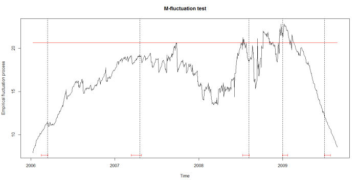
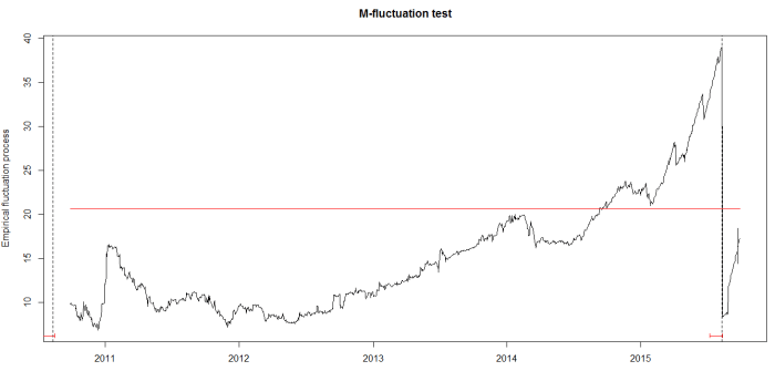
	## plot LM statistics along with confidence interval
	flm_rep <- fxlm(CNY ~ USD + JPY + EUR + GBP, data = cny_rep)
	scus_rep <- gefp(flm_rep, fit = NULL)
	plot(scus_rep, functional = supLM(0.1))
	## add lines related to breaks to your plot
	lines(cit_rep)

	apply(cny_rep,1,function(x) sum(is.na(x)))

view raw FrankelWei_2010_2016.r hosted with ❤ by GitHub

We got breaks in 2010 and in 2015 (when China’s stock markets crashed). We would have hoped for more breaks (we can still get them), but that would depend on the parameters chosen for our regression.

Google’s New Deep Learning MOOC Using TensorFlow

January 24, 2016 Anirudh Technical Deep Learning, IPython, Machine Learning, MOOC, TensorFlow, Udacity

Deep learning became a hot topic in machine learning in the last 3-4 years (see inset below) and recently, Google released TensorFlow (a Python based deep learning toolkit) as an open source project to bring deep learning to everyone.

deep_learning_google_trends — Interest in the Google search term *Deep Learning* over time

If you have wanted to get your hands dirty with TensorFlow or needed more direction with that, here’s some good news – Google is offering an open MOOC on deep learning methods using TensorFlow here. This course has been developed with Vincent Vanhoucke, Principal Scientist at Google, and technical lead in the Google Brain team. However, this is an intermediate to advanced level course and assumes you have taken a first course in machine learning, or that you are at least familiar with supervised learning methods.

Google’s overall goal in designing this course is to provide the machine learning enthusiast a rapid and direct path to solving real and interesting problems with deep learning techniques.

What is Deep Learning?