Endogenously Detecting Structural Breaks in a Time Series: Implementation in R

The most conventional approach to determine structural breaks in longitudinal data seems to be the Chow Test.

From Wikipedia,

The Chow test, proposed by econometrician Gregory Chow in 1960, is a test of whether the coefficients in two linear regressions on different data sets are equal. In econometrics, it is most commonly used in time series analysis to test for the presence of a structural break at a period which can be assumed to be known a priori (for instance, a major historical event such as a war). In program evaluation, the Chow test is often used to determine whether the independent variables have different impacts on different subgroups of the population.

As shown in the figure below, regressions on the 2 sub-intervals seem to have greater explanatory power than a single regression over the data.

440px-chow_test_structural_break

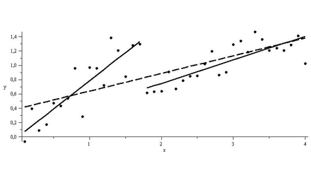
For the data above, determining the sub-intervals is an easy task. However, things may not look that simple in reality. Conducting a Chow test for structural breaks leaves the data scientist at the mercy of his subjective gaze in choosing a null hypothesis for a break point in the data.

Instead of choosing the breakpoints in an exogenous manner, what if the data itself could learn where these breakpoints lie? Such an endogenous technique is what Bai and Perron came up with in a seminal paper published in 1998 that could detect multiple structural breaks in longitudinal data. A later paper in 2003 dealt with the testing for breaks empirically, using a dynamic programming algorithm based on the Bellman principle.

I will discuss a quick implementation of this technique in R.

Brief Outline:

Assuming you have a ts object (I don’t know whether this works with zoo, but it should) in R, called ts. Then implement the following:

# assuming you have a 'ts' object in R
# 1. install package 'strucchange'
# 2. Then write down this code:
library(strucchange)
# store the breakdates
bp_ts <- breakpoints(ts ~ 1)
# this will give you the break dates and their confidence intervals
summary(bp_ts)
# store the confidence intervals
ci_ts <- confint(bp_ts)
## to plot the breakpoints with confidence intervals
plot(ts)
lines(bp_ts)
lines(ci_ts)

An illustration 

I started with data on India’s rice crop productivity between 1950 (around Independence from British Colonial rule) and 2008. Here’s how it looks:

rice_productivity

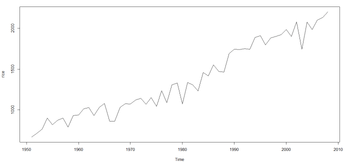
You can download the excel and CSV files here and here respectively.

Here’s the way to go using R:

library(xlsx)
library(forecast)
library(tseries)
library(strucchange)
## load the data from a CSV or Excel file. This example is done with an Excel sheet.
prod_df <- read.xlsx(file = 'agricultural_productivity.xls', sheetIndex = 'Sheet1', rowIndex = 8:65, colIndex = 2, header = FALSE)
colnames(prod_df) <- c('Rice')
## store rice data as time series objects
rice <- ts(prod_df$Rice, start=c(1951, 1), end=c(2008, 1), frequency=1)
# store the breakpoints
bp.rice <- breakpoints(rice ~ 1)
summary(bp.rice)
## the BIC chooses 5 breakpoints; plot the graph with breakdates and their confidence intervals
plot(bp.rice)
plot(rice)
lines(bp.rice)
## confidence intervals
ci.rice <- confint(bp.rice)
ci.rice
lines(ci.rice)

Voila, this is what you get:

02_rice_multiplebreaks

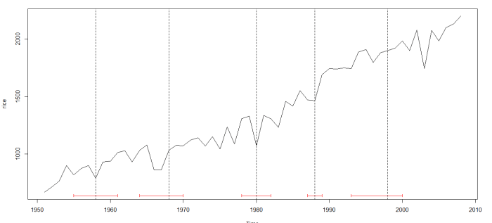
The dotted vertical lines indicated the break dates; the horizontal red lines indicate their confidence intervals.

This is a quick and dirty implementation. For a more detailed take, check out the documentation on the R package called strucchange.

Abu Mostafa’s Machine Learning MOOC – Now on EdX

This was in the pipeline for quite some time now. I have been waiting for his lectures on a platform such as EdX or Coursera, and the day has arrived. You can enroll and start with week 1’s lectures as they’re live now.

This course is taught by none other than Dr. Yaser S. Abu – Mostafa, whose textbook on machine learning, Learning from Data is #1 bestseller textbook (Amazon) in all categories of Computer Science. His online course has been offered earlier over here.

Teaching

Dr. Abu-Mostafa received the Clauser Prize for the most original doctoral thesis at Caltech. He received the ASCIT Teaching Awards in 1986, 1989 and 1991, the GSC Teaching Awards in 1995 and 2002, and the Richard P. Feynman prize for excellence in teaching in 1996.

Live ‘One-take’ Recordings

The lectures have been recorded from a live broadcast (including Q&A, which will let you gauge the level of CalTech students taking this course). In fact, it almost seems as though Abu Mostafa takes a direct jab at Andrew Ng’s popular Coursera MOOC by stating the obvious on his course page.

A real Caltech course, not a watered-down version

screenshot-www-work-caltech-edu-2016-09-24-22-19-21

Again, while enrolling note that this is what Abu Mostafa had to say about the online course:  “A Caltech course does not cater to short attention spans, and it may not provide instant gratification…[like] many MOOCs out there that are quite simple and have a ‘video game’ feel to them.” Unsurprisingly, many online students have dropped out in the past, but some of those students who “complained early on but decided to stick with the course had very flattering words to say at the end”.

Prerequisites

  • Basic probability
  • Basic matrices
  • Basic calculus
  • Some programming language/platform (I choose Python!)

If you’re looking for a challenging machine learning course, this is probably one you must take.


MITx: 6.008.1x Computational Probability and Inference

I got really interested in Computational Probability and Inference (6.008.1x) for the following reasons:

  1. I love probability and have solved countless problems on probability ever since I learned math
  2. …and yet I’ve never coded up probabilistic models!
  3. The assignments and project work for this course are to be implemented in Python!

You don’t need to have prior experience in either probability or inference, but you should be comfortable with basic Python programming and calculus.

WHAT YOU’LL LEARN
– Basic discrete probability theory
– Graphical models as a data structure for representing probability distributions
– Algorithms for prediction and inference
– How to model real-world problems in terms of probabilistic inference

The course started on September 12, is 12-weeks long and is structured in the following manner:

Week 1 (9/12 – 9/16): Introduction to probability and computation
A first look at basic discrete probability, how to interpret it, what probability spaces and random variables are, and how to code these up and do basic simulations and visualizations.

Week 2 (9/19 – 9/23): Incorporating observations
Incorporating observations using jointly distributed random variables and using events. Three classic probability puzzles are presented to help elucidate how to interpret probability: Simpson’s paradox, Monty Hall, boy or girl paradox.

Week 3 (9/26 – 9/30): Introduction to inference, structure in distributions, and information measures
The product rule and inference with Bayes’ theorem. Independence: A structure in distributions. Measures of randomness: entropy and information divergence. Mutual information.

Week 4 (10/3 – 10/7): Expectations, and driving to infinity in modeling uncertainty
Expected values of random variables. Classic puzzle: the two envelope problem. Probability spaces and random variables that take on a countably infinite number of values and inference with these random variables.

Week 5 (10/10 – 10/14): Efficient representations of probability distributions on a computer
Introduction to undirected graphical models as a data structure for representing probability distributions and the benefits/drawbacks of these graphical models. Incorporating observations with graphical models.

Week 6 (10/17 – 10/21): Inference with graphical models, part I
Computing marginal distributions with graphical models in undirected graphical models including hidden Markov models..

Week 7 (10/24 – 10/28): Inference with graphical models, part II
Computing most probable configurations with graphical models including hidden Markov models.

Week 8 (10/31 – 11/4): Introduction to learning probability distributions
Learning an underlying unknown probability distribution from observations using maximum likelihood. Three examples: estimating the bias of a coin, the German tank problem, and email spam detection.

Week 9 (11/7 – 11/11): Parameter estimation in graphical models
Given the graph structure of an undirected graphical model, we examine how to estimate all the tables associated with the graphical model.

Week 10 (11/14 – 11/18): Model selection with information theory
Learning both the graph structure and the tables of an undirected graphical model with the help of information theory. Mutual information of random variables.

Week 11 (11/21 – 11/25): Final project
Final project assigned

Week 12 (11/28 – 12/2): Final project


I’m SO taking this course. Hope this interests you as well!

Analytics Vidhya Workshop / Hackathon – Experiments with Data

This was a hackathon + workshop conducted by Analytics Vidhya in which I took part and made it to the #1 on the leaderboard. The data set was straight-forward and quite clean with only a minor need for missing value treatment. This post will might be useful for people who want a walk-through on the steps involving data munging and developing machine-learned models.

screenshot-datahack.analyticsvidhya.com 2016-09-01 23-43-54


The workshop ended with a basic hackathon with data given on age, education, working class, occupation, marital status and gender of individuals and one had to predict the income bracket of these individuals.

I’ve posted the data and my code and solutions in this GitHub repo. An IPython Notebook has also been shared.

I approached the problem first by attempting some feature engineering (other than missing value treatment) on the data, and then ran a basic logistic classifier and a random forest classifier. However it turned out that these models performed better without feature engineering, which shows the dataset was already quite clean and informative to begin with for this competition.

I later attempted gradient boosting with parameter tuning to maximizing scores.

Loading
Sorry, something went wrong. Reload?
Sorry, we cannot display this file.
Sorry, this file is invalid so it cannot be displayed.

Implementing Undirected Graphs in Python

There are 2 popular ways of representing an undirected graph.

Adjacency List
Each list describes the set of neighbors of a vertex in the graph.

adjacencyList

Adjacency Matrix
The elements of the matrix indicate whether pairs of vertices are adjacent or not in the graph.

adjacencyMatrix

Here’s an implementation of the above in Python:

class Vertex:
def __init__(self, vertex):
self.name = vertex
self.neighbors = []
def add_neighbor(self, neighbor):
if isinstance(neighbor, Vertex):
if neighbor.name not in self.neighbors:
self.neighbors.append(neighbor.name)
neighbor.neighbors.append(self.name)
self.neighbors = sorted(self.neighbors)
neighbor.neighbors = sorted(neighbor.neighbors)
else:
return False
def add_neighbors(self, neighbors):
for neighbor in neighbors:
if isinstance(neighbor, Vertex):
if neighbor.name not in self.neighbors:
self.neighbors.append(neighbor.name)
neighbor.neighbors.append(self.name)
self.neighbors = sorted(self.neighbors)
neighbor.neighbors = sorted(neighbor.neighbors)
else:
return False
def __repr__(self):
return str(self.neighbors)
class Graph:
def __init__(self):
self.vertices = {}
def add_vertex(self, vertex):
if isinstance(vertex, Vertex):
self.vertices[vertex.name] = vertex.neighbors
def add_vertices(self, vertices):
for vertex in vertices:
if isinstance(vertex, Vertex):
self.vertices[vertex.name] = vertex.neighbors
def add_edge(self, vertex_from, vertex_to):
if isinstance(vertex_from, Vertex) and isinstance(vertex_to, Vertex):
vertex_from.add_neighbor(vertex_to)
if isinstance(vertex_from, Vertex) and isinstance(vertex_to, Vertex):
self.vertices[vertex_from.name] = vertex_from.neighbors
self.vertices[vertex_to.name] = vertex_to.neighbors
def add_edges(self, edges):
for edge in edges:
self.add_edge(edge[0],edge[1])
def adjacencyList(self):
if len(self.vertices) >= 1:
return [str(key) + ":" + str(self.vertices[key]) for key in self.vertices.keys()]
else:
return dict()
def adjacencyMatrix(self):
if len(self.vertices) >= 1:
self.vertex_names = sorted(g.vertices.keys())
self.vertex_indices = dict(zip(self.vertex_names, range(len(self.vertex_names))))
import numpy as np
self.adjacency_matrix = np.zeros(shape=(len(self.vertices),len(self.vertices)))
for i in range(len(self.vertex_names)):
for j in range(i, len(self.vertices)):
for el in g.vertices[self.vertex_names[i]]:
j = g.vertex_indices[el]
self.adjacency_matrix[i,j] = 1
return self.adjacency_matrix
else:
return dict()
def graph(g):
""" Function to print a graph as adjacency list and adjacency matrix. """
return str(g.adjacencyList()) + '\n' + '\n' + str(g.adjacencyMatrix())
###################################################################################
a = Vertex('A')
b = Vertex('B')
c = Vertex('C')
d = Vertex('D')
e = Vertex('E')
a.add_neighbors([b,c,e])
b.add_neighbors([a,c])
c.add_neighbors([b,d,a,e])
d.add_neighbor(c)
e.add_neighbors([a,c])
g = Graph()
print(graph(g))
print()
g.add_vertices([a,b,c,d,e])
g.add_edge(b,d)
print(graph(g))

Output:

{}
{}
["A:['B', 'C', 'E']", "C:['A', 'B', 'D', 'E']", "B:['A', 'C', 'D']", "E:['A', 'C']", "D:['B', 'C']"]
[[ 0. 1. 1. 0. 1.]
[ 1. 0. 1. 1. 0.]
[ 1. 1. 0. 1. 1.]
[ 0. 1. 1. 0. 0.]
[ 1. 0. 1. 0. 0.]]

Deterministic Selection Algorithm Python Code

Through this post, I’m sharing Python code implementing the median of medians algorithm, an algorithm that resembles quickselect, differing only in the way in which the pivot is chosen, i.e, deterministically, instead of at random.

Its best case complexity is O(n) and worst case complexity O(nlog2n)

I don’t have a formal education in CS, and came across this algorithm while going through Tim Roughgarden’s Coursera MOOC on the design and analysis of algorithms. Check out my implementation in Python.

def merge_tuple(a,b):
""" Function to merge two arrays of tuples """
c = []
while len(a) != 0 and len(b) != 0:
if a[0][0] < b[0][0]:
c.append(a[0])
a.remove(a[0])
else:
c.append(b[0])
b.remove(b[0])
if len(a) == 0:
c += b
else:
c += a
return c
def mergesort_tuple(x):
""" Function to sort an array using merge sort algorithm """
if len(x) == 0 or len(x) == 1:
return x
else:
middle = len(x)/2
a = mergesort_tuple(x[:middle])
b = mergesort_tuple(x[middle:])
return merge_tuple(a,b)
def lol(x,k):
""" Function to divide a list into a list of lists of size k each. """
return [x[i:i+k] for i in range(0,len(x),k)]
def preprocess(x):
""" Function to assign an index to each element of a list of integers, outputting a list of tuples"""
return zip(x,range(len(x)))
def partition(x, pivot_index = 0):
""" Function to partition an unsorted array around a pivot"""
i = 0
if pivot_index !=0: x[0],x[pivot_index] = x[pivot_index],x[0]
for j in range(len(x)-1):
if x[j+1] < x[0]:
x[j+1],x[i+1] = x[i+1],x[j+1]
i += 1
x[0],x[i] = x[i],x[0]
return x,i
def ChoosePivot(x):
""" Function to choose pivot element of an unsorted array using 'Median of Medians' method. """
if len(x) <= 5:
return mergesort_tuple(x)[middle_index(x)]
else:
lst = lol(x,5)
lst = [mergesort_tuple(el) for el in lst]
C = [el[middle_index(el)] for el in lst]
return ChoosePivot(C)
def DSelect(x,k):
""" Function to """
if len(x) == 1:
return x[0]
else:
xpart = partition(x,ChoosePivot(preprocess(x))[1])
x = xpart[0] # partitioned array
j = xpart[1] # pivot index
if j == k:
return x[j]
elif j > k:
return DSelect(x[:j],k)
else:
k = k - j - 1
return DSelect(x[(j+1):], k)
arr = range(100,0,-1)
print DSelect(arr,50)
%timeit DSelect(arr,50)
view raw DSelect.py hosted with ❤ by GitHub

I get the following output:

51
100 loops, best of 3: 2.38 ms per loop

Note that on the same input, quickselect is faster, giving us:

1000 loops, best of 3: 254 µs per loop

scikit-learn Linear Regression Example

Here’s a quick example case for implementing one of the simplest of learning algorithms in any machine learning toolbox – Linear Regression. You can download the IPython / Jupyter notebook here so as to play around with the code and try things out yourself.

I’m doing a series of posts on scikit-learn. Its documentation is vast, so unless you’re willing to search for a needle in a haystack, you’re better off NOT jumping into the documentation right away. Instead, knowing chunks of code that do the job might help.

Loading
Sorry, something went wrong. Reload?
Sorry, we cannot display this file.
Sorry, this file is invalid so it cannot be displayed.

Sharing IPython / Jupyter Notebooks via WordPress

In order to share (a static version of) your IPython / Jupyter notebook on your WordPress site, follow three straightforward steps.

Step 1: Let’s say your Jupyter Notebook looks like this:

blog_item_20160718_01

Open this notebook in a text editor and copy the content which may look like so:

blog_item_20160718_02

Step 2: Ctrl + A and Ctrl + C this content. Then Ctrl + V this to a GitHub Gist that you should create, like so:

blog_item_20160718_03

Step 3: Now simply Create public gist and embed the gist like you always embed gists on WordPress, viz., go to the HTML editor and add like so:

blog_item_20160718_04

I followed the exact steps that I’ve mentioned above to get the following result:

Loading
Sorry, something went wrong. Reload?
Sorry, we cannot display this file.
Sorry, this file is invalid so it cannot be displayed.
view raw knn.ipynb hosted with ❤ by GitHub


Randomized Selection Algorithm (Quickselect) – Python Code

Find the kth smallest element in an array without sorting.

That’s basically what this algorithm does. It piggybacks on the partition subroutine from the Quick Sort. If you don’t know what that is, you can check out more about the Quick Sort algorithm here and here, and understand the usefulness of partitioning an unsorted array around a pivot.

Selecting_quickselect_frames
Animated visualization of the randomized selection algorithm selecting the 22nd
smallest value

Python Implementation

from random import randrange
def partition(x, pivot_index = 0):
i = 0
if pivot_index !=0: x[0],x[pivot_index] = x[pivot_index],x[0]
for j in range(len(x)-1):
if x[j+1] < x[0]:
x[j+1],x[i+1] = x[i+1],x[j+1]
i += 1
x[0],x[i] = x[i],x[0]
return x,i
def RSelect(x,k):
if len(x) == 1:
return x[0]
else:
xpart = partition(x,randrange(len(x)))
x = xpart[0] # partitioned array
j = xpart[1] # pivot index
if j == k:
return x[j]
elif j > k:
return RSelect(x[:j],k)
else:
k = k - j - 1
return RSelect(x[(j+1):], k)
x = [3,1,8,4,7,9]
for i in range(len(x)):
print RSelect(x,i),
view raw RSelect.py hosted with ❤ by GitHub


Related Posts
Quick Sort Python Code
Computing Work Done (Total Pivot Comparisons) by Quick Sort

Computing Work Done (Total Pivot Comparisons) by Quick Sort

A key aspect of the Quick Sort algorithm is how the pivot element is chosen. In my earlier post on the Python code for Quick Sort, my implementation takes the first element of the unsorted array as the pivot element.

However with some mathematical analysis it can be seen that such an implementation is O(n2) in complexity while if a pivot is randomly chosen, the Quick Sort algorithm is O(nlog2n).

To witness this in action, one can measure the work done by the algorithm comparing two cases, one with a randomized pivot choice – and one with a fixed pivot choice, say the first element of the array (or the last element of the array).

Implementation

A decent proxy for the amount of work done by the algorithm would be the number of pivot comparisons. These comparisons needn’t be computed one-by-one, rather when there is a recursive call on a subarray of length m, you should simply add m−1 to your running total of comparisons.

3 Cases

To put things in perspective, let’s look at 3 cases. (This is basically straight out of a homework assignment from Tim Roughgarden’s course on the Design and Analysis of Algorithms).
Case I with the pivot being the first element.
Case II with the pivot being the last element.
Case III using the “median-of-three” pivot rule. The primary motivation behind this rule is to do a little bit of extra work to get much better performance on input arrays that are nearly sorted or reverse sorted.

Median-of-Three Pivot Rule

Consider the first, middle, and final elements of the given array. (If the array has odd length it should be clear what the “middle” element is; for an array with even length 2k, use the kth element as the “middle” element. So for the array 4 5 6 7, the “middle” element is the second one —- 5 and not 6! Identify which of these three elements is the median (i.e., the one whose value is in between the other two), and use this as your pivot.

Python Code

This file contains all of the integers between 1 and 10,000 (inclusive, with no repeats) in unsorted order. The integer in the ith row of the file gives you the ith entry of an input array. I downloaded this file and named it QuickSort_List.txt

You can run the code below and see for yourself that the number of comparisons for Case III are 138,382 compared to 162,085 and 164,123 for Case I and Case II respectively. You can play around with the code in an IPython / Jupyter notebook here.

#!/usr/bin/env
# Case I
# First element of the unsorted array is chosen as pivot element for sorting using Quick Sort
def countComparisonsWithFirst(x):
""" Counts number of comparisons while using Quick Sort with first element of unsorted array as pivot """
global count_pivot_first
if len(x) == 1 or len(x) == 0:
return x
else:
count_pivot_first += len(x)-1
i = 0
for j in range(len(x)-1):
if x[j+1] < x[0]:
x[j+1],x[i+1] = x[i+1], x[j+1]
i += 1
x[0],x[i] = x[i],x[0]
first_part = countComparisonsWithFirst(x[:i])
second_part = countComparisonsWithFirst(x[i+1:])
first_part.append(x[i])
return first_part + second_part
# Case II
# Last element of the unsorted array is chosen as pivot element for sorting using Quick Sort
def countComparisonsWithLast(x):
""" Counts number of comparisons while using Quick Sort with last element of unsorted array as pivot """
global count_pivot_last
if len(x) == 1 or len(x) == 0:
return x
else:
count_pivot_last += len(x)-1
x[0],x[-1] = x[-1],x[0]
i = 0
for j in range(len(x)-1):
if x[j+1] < x[0]:
x[j+1],x[i+1] = x[i+1], x[j+1]
i += 1
x[0],x[i] = x[i],x[0]
first_part = countComparisonsWithLast(x[:i])
second_part = countComparisonsWithLast(x[i+1:])
first_part.append(x[i])
return first_part + second_part
# Case III
# Median-of-three method used to choose pivot element for sorting using Quick Sort
def middle_index(x):
""" Returns the index of the middle element of an array """
if len(x) % 2 == 0:
middle_index = len(x)/2 - 1
else:
middle_index = len(x)/2
return middle_index
def median_index(x,i,j,k):
""" Returns the median index of three when passed an array and indices of any 3 elements of that array """
if (x[i]-x[j])*(x[i]-x[k]) < 0:
return i
elif (x[j]-x[i])*(x[j]-x[k]) < 0:
return j
else:
return k
def countComparisonsMedianOfThree(x):
""" Counts number of comparisons while using Quick Sort with median-of-three element is chosen as pivot """
global count_pivot_median
if len(x) == 1 or len(x) == 0:
return x
else:
count_pivot_median += len(x)-1
k = median_index(x, 0, middle_index(x), -1)
if k != 0: x[0], x[k] = x[k], x[0]
i = 0
for j in range(len(x)-1):
if x[j+1] < x[0]:
x[j+1],x[i+1] = x[i+1], x[j+1]
i += 1
x[0],x[i] = x[i],x[0]
first_part = countComparisonsMedianOfThree(x[:i])
second_part = countComparisonsMedianOfThree(x[i+1:])
first_part.append(x[i])
return first_part + second_part
#####################################################################
# initializing counts
count_pivot_first = 0; count_pivot_last = 0; count_pivot_median = 0
#####################################################################
# Cast I
# Read the contents of the file into a Python list
NUMLIST_FILENAME = "QuickSort_List.txt"
inFile = open(NUMLIST_FILENAME, 'r')
with inFile as f: numList = [int(integers.strip()) for integers in f.readlines()]
# call functions to count comparisons
countComparisonsWithFirst(numList)
#####################################################################
# Read the contents of the file into a Python list
NUMLIST_FILENAME = "QuickSort_List.txt"
inFile = open(NUMLIST_FILENAME, 'r')
with inFile as f: numList = [int(integers.strip()) for integers in f.readlines()]
# call functions to count comparisons
countComparisonsWithLast(numList)
#####################################################################
# Read the contents of the file into a Python list
NUMLIST_FILENAME = "QuickSort_List.txt"
inFile = open(NUMLIST_FILENAME, 'r')
with inFile as f: numList = [int(integers.strip()) for integers in f.readlines()]
# call functions to count comparisons
countComparisonsMedianOfThree(numList)
#####################################################################
print count_pivot_first, count_pivot_last, count_pivot_median