Scraping the Daily India Covid-19 Tracker for CSV Data

This is a very short post that will be very useful to help you quickly set up your COVID-19 datasets. I’m sharing code at the end of this post that scrapes through all CSV datasets made available by COVID19-India API.

Copy paste this standalone script into your R environment and get going!

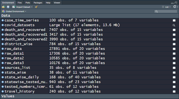
There are 15+ CSV files on the India COVID-19 API website. raw_data3 is actually a live dataset and more can be expected in the days to come, which is why a script that automates the data sourcing comes in handy.  Snapshot of the file names and the data dimensions as of today, 100 days since the first case was recorded in the state of Kerala —

Image

My own analysis of the data and predictions are work-in-progress, going into a Github repo. Execute the code below and get started analyzing the data and fighting COVID-19!

rm(list = ls())
# Load relevant libraries -----------------------------------------------------
library(stringr)
library(data.table)
# =============================================================================
# COVID 19-India API: A volunteer-driven, crowdsourced database
# for COVID-19 stats & patient tracing in India
# =============================================================================
url <- "https://api.covid19india.org/csv/&quot;
# List out all CSV files to source --------------------------------------------
html <- paste(readLines(url), collapse="\n")
pattern <- "https://api.covid19india.org/csv/latest/.*csv&quot;
matched <- unlist(str_match_all(string = html, pattern = pattern))
# Downloading the Data --------------------------------------------------------
covid_datasets <- lapply(as.list(matched), fread)
# Naming the data objects appropriately ---------------------------------------
exclude_chars <- "https://api.covid19india.org/csv/latest/&quot;
dataset_names <- substr(x = matched,
start = 1 + nchar(exclude_chars),
stop = nchar(matched)- nchar(".csv"))
# assigning variable names
for(i in seq_along(dataset_names)){
assign(dataset_names[i], covid_datasets[[i]])
}

Linear Algebra behind the lm() function in R

This post comes out of the blue, nearly 2 years since my last one. I realize I’ve been lazy, so here’s hoping I move from an inertia of rest to that of motion, implying, regular and (hopefully) relevant posts. I also chanced upon some wisdom while scrolling through my Twitter feed:

This blog post in particular was meant to be a reminder to myself and other R users that the much used lm() function in R (for fitting linear models) can be replaced with some handy matrix operations to obtain regression coefficients, their standard errors and other goodness-of-fit stats printed out when summary() is called on an lm object.

Linear regression can be formulated mathematically as follows:
\mathbf{y} = \mathbf{X} \mathbf{\beta} + \mathbf{\epsilon} ,
\mathbf{\epsilon} \sim N(0, \sigma^2 \mathbf{I})

\mathbf{y} is the \mathbf{n}\times \mathbf{1} outcome variable and \mathbf{X} is the \mathbf{n}\times \mathbf{(\mathbf{k}+1)} data matrix of independent predictor variables (including a vector of ones corresponding to the intercept). The ordinary least squares (OLS) estimate for the vector of coefficients \mathbf{\beta} is:

\hat{\mathbf{\beta}} = (\mathbf{X}^{\prime} \mathbf{X})^{-1} \mathbf{X}^{\prime} \mathbf{y}

The covariance matrix can be obtained with some handy matrix operations:
\textrm{Var}(\hat{\mathbf{\beta}}) = (\mathbf{X}^{\prime} \mathbf{X})^{-1} \mathbf{X}^{\prime} \;\sigma^2 \mathbf{I} \; \mathbf{X} (\mathbf{X}^{\prime} \mathbf{X})^{-1} = \sigma^2 (\mathbf{X}^{\prime} \mathbf{X})^{-1}
given that \textrm{Var}(AX) = A \times \textrm{Var}X \times A^{\prime}; \textrm{Var}(\mathbf{y}) = \mathbf{\sigma^2}

The standard errors of the coefficients are basically \textrm{Diag}(\sqrt{\textrm{Var}(\hat{\mathbf{\beta}})}) = \textrm{Diag}(\sqrt{\sigma^2 (\mathbf{X}^{\prime} \mathbf{X})^{-1}}) and with these, one can compute the t-statistics and their corresponding p-values.

Lastly, the F-statistic and its corresponding p-value can be calculated after computing the two residual sum of squares (RSS) statistics:

  • \mathbf{RSS} – for the full model with all predictors
  • \mathbf{RSS_0} – for the partial model (\mathbf{y} = \mathbf{\mu} + \mathbf{\nu}; \mathbf{\mu} = \mathop{\mathbb{E}}[\mathbf{y}]; \mathbf{\nu} \sim N(0, \sigma_0^2 \mathbf{I}) ) with the outcome observed mean as estimated outcome

\mathbf{F} = \frac{(\mathbf{RSS_0}-\mathbf{RSS})/\mathbf{k}}{\mathbf{RSS}/(\mathbf{n}-\mathbf{k}-1)}

I wrote some R code to construct the output from summarizing lm objects, using all the math spewed thus far. The data used for this exercise is available in R, and comprises of standardized fertility measures and socio-economic indicators for each of 47 French-speaking provinces of Switzerland from 1888. Try it out and see for yourself the linear algebra behind linear regression.

### Linear Regression Using lm() ----------------------------------------
data("swiss")
dat <- swiss
linear_model <- lm(Fertility ~ ., data = dat)
summary(linear_model)
# Call:
# lm(formula = Fertility ~ ., data = dat)
#
# Residuals:
# Min 1Q Median 3Q Max
# -15.2743 -5.2617 0.5032 4.1198 15.3213
#
# Coefficients:
# Estimate Std. Error t value Pr(>|t|)
# (Intercept) 66.91518 10.70604 6.250 1.91e-07 ***
# Agriculture -0.17211 0.07030 -2.448 0.01873 *
# Examination -0.25801 0.25388 -1.016 0.31546
# Education -0.87094 0.18303 -4.758 2.43e-05 ***
# Catholic 0.10412 0.03526 2.953 0.00519 **
# Infant.Mortality 1.07705 0.38172 2.822 0.00734 **
# ---
# Signif. codes: 0 ‘***’ 0.001 ‘**’ 0.01 ‘*’ 0.05 ‘.’ 0.1 ‘ ’ 1
#
# Residual standard error: 7.165 on 41 degrees of freedom
# Multiple R-squared: 0.7067, Adjusted R-squared: 0.671
# F-statistic: 19.76 on 5 and 41 DF, p-value: 5.594e-10
### Using Linear Algebra ------------------------------------------------
y <- matrix(dat$Fertility, nrow = nrow(dat))
X <- cbind(1, as.matrix(x = dat[,-1]))
colnames(X)[1] <- "(Intercept)"
# N x k matrix
N <- nrow(X)
k <- ncol(X) - 1 # number of predictor variables (ergo, excluding Intercept column)
# Estimated Regression Coefficients
beta_hat <- solve(t(X)%*%X)%*%(t(X)%*%y)
# Variance of outcome variable = Variance of residuals
sigma_sq <- residual_variance <- (N-k-1)^-1 * sum((y - X %*% beta_hat)^2)
residual_std_error <- sqrt(residual_variance)
# Variance and Std. Error of estimated coefficients of the linear model
var_betaHat <- sigma_sq * solve(t(X) %*% X)
coeff_std_errors <- sqrt(diag(var_betaHat))
# t values of estimates are ratio of estimated coefficients to std. errors
t_values <- beta_hat / coeff_std_errors
# p-values of t-statistics of estimated coefficeints
p_values_tstat <- 2 * pt(abs(t_values), N-k, lower.tail = FALSE)
# assigning R's significance codes to obtained p-values
signif_codes_match <- function(x){
ifelse(x <= 0.001,"***",
ifelse(x <= 0.01,"**",
ifelse(x < 0.05,"*",
ifelse(x < 0.1,"."," "))))
}
signif_codes <- sapply(p_values_tstat, signif_codes_match)
# R-squared and Adjusted R-squared (refer any econometrics / statistics textbook)
R_sq <- 1 - (N-k-1)*residual_variance / (N*mean((y - mean(y))^2))
R_sq_adj <- 1 - residual_variance / ((N/(N-1))*mean((y - mean(y))^2))
# Residual sum of squares (RSS) for the full model
RSS <- (N-k-1)*residual_variance
# RSS for the partial model with only intercept (equal to mean), ergo, TSS
RSS0 <- TSS <- sum((y - mean(y))^2)
# F statistic based on RSS for full and partial models
# k = degress of freedom of partial model
# N - k - 1 = degress of freedom of full model
F_stat <- ((RSS0 - RSS)/k) / (RSS/(N-k-1))
# p-values of the F statistic
p_value_F_stat <- pf(F_stat, df1 = k, df2 = N-k-1, lower.tail = FALSE)
# stitch the main results toghether
lm_results <- as.data.frame(cbind(beta_hat, coeff_std_errors,
t_values, p_values_tstat, signif_codes))
colnames(lm_results) <- c("Estimate","Std. Error","t value","Pr(>|t|)","")
### Print out results of all relevant calcualtions -----------------------
print(lm_results)
cat("Residual standard error: ",
round(residual_std_error, digits = 3),
" on ",N-k-1," degrees of freedom",
"\nMultiple R-squared: ",R_sq," Adjusted R-squared: ",R_sq_adj,
"\nF-statistic: ",F_stat, " on ",k-1," and ",N-k-1,
" DF, p-value: ", p_value_F_stat,"\n")
# Estimate Std. Error t value Pr(>|t|)
# (Intercept) 66.9151816789654 10.7060375853301 6.25022854119771 1.73336561301153e-07 ***
# Agriculture -0.172113970941457 0.0703039231786469 -2.44814177018405 0.0186186100433133 *
# Examination -0.258008239834722 0.253878200892098 -1.01626779663678 0.315320687313066
# Education -0.870940062939429 0.183028601571259 -4.75849159892283 2.3228265226988e-05 ***
# Catholic 0.104115330743766 0.035257852536169 2.95296858017545 0.00513556154915653 **
# Infant.Mortality 1.07704814069103 0.381719650858061 2.82156849475775 0.00726899472564356 **
# Residual standard error: 7.165 on 41 degrees of freedom
# Multiple R-squared: 0.706735 Adjusted R-squared: 0.670971
# F-statistic: 19.76106 on 4 and 41 DF, p-value: 5.593799e-10

Hope this was useful and worth your time!

Installing Tensorflow on Windows is Easy!

I recently got myself to start using Python on Windows, whereas till very recently I had been working on Python only from Ubuntu.

I am sure I am late in realizing this, but installing Tensorflow was just so easy!

If you’ve tried installing Tensorflow for Windows when it was first introduced, and gave up back then – try again. The method I’d recommend would be using Anaconda Navigator from where you first open a terminal (figure below). You may notice that I already have a tensorflow environment set up, since I am writing this post after installation.

anaconda navigator

Once you have terminal open, create a conda environment named tensorflow by invoking the following command, with your python version:

C:> conda create -n tensorflow python=3.6

That’s all! You should now have tensorflow ready to use.

For more details, you could always go here. Otherwise, the screenshot below gives a sense of what it takes.

tensorflow installed


Linear / Logistic Regression in R: Dealing With Unknown Factor Levels in Test Data

Let’s say you have data containing a categorical variable with 50 levels. When you divide the data into train and test sets, chances are you don’t have all 50 levels featuring in your training set.

This often happens when you divide the data set into train and test sets according to the distribution of the outcome variable. In doing so, chances are that our explanatory categorical variable might not be distributed exactly the same way in train and test sets – so much so that certain levels of this categorical variable are missing from the training set. The more levels there are to a categorical variable, it gets difficult for that variable to be similarly represented upon splitting the data.

Take for instance this example data set (train.csv + test.csv) which contains a categorical variable var_b that takes 349 unique levels. Our train data has 334 of these levels – on which the model is built – and hence 15 levels are excluded from our trained model. If you try making predictions on the test set with this model in R, it throws an error:
factor var_b has new levels 16060, 17300, 17980, 19060, 21420, 21820,
25220, 29340, 30300, 33260, 34100, 38340, 39660, 44300, 45460

If you’ve used R to model generalized linear class of models such as linear, logit or probit models, then chances are you’ve come across this problem – especially when you’re validating your trained model on test data.

The workaround to this problem is in the form of a function, remove_missing_levels  that I found here written by pat-s. You need magrittr library installed and it can only work on lm, glm and glmmPQL objects.

remove_missing_levels <- function(fit, test_data) {
library(magrittr)
# https://stackoverflow.com/a/39495480/4185785
# drop empty factor levels in test data
test_data %>%
droplevels() %>%
as.data.frame() -> test_data
# 'fit' object structure of 'lm' and 'glmmPQL' is different so we need to
# account for it
if (any(class(fit) == "glmmPQL")) {
# Obtain factor predictors in the model and their levels
factors <- (gsub("[-^0-9]|as.factor|\\(|\\)", "",
names(unlist(fit$contrasts))))
# do nothing if no factors are present
if (length(factors) == 0) {
return(test_data)
}
map(fit$contrasts, function(x) names(unmatrix(x))) %>%
unlist() -> factor_levels
factor_levels %>% str_split(":", simplify = TRUE) %>%
extract(, 1) -> factor_levels
model_factors <- as.data.frame(cbind(factors, factor_levels))
} else {
# Obtain factor predictors in the model and their levels
factors <- (gsub("[-^0-9]|as.factor|\\(|\\)", "",
names(unlist(fit$xlevels))))
# do nothing if no factors are present
if (length(factors) == 0) {
return(test_data)
}
factor_levels <- unname(unlist(fit$xlevels))
model_factors <- as.data.frame(cbind(factors, factor_levels))
}
# Select column names in test data that are factor predictors in
# trained model
predictors <- names(test_data[names(test_data) %in% factors])
# For each factor predictor in your data, if the level is not in the model,
# set the value to NA
for (i in 1:length(predictors)) {
found <- test_data[, predictors[i]] %in% model_factors[
model_factors$factors == predictors[i], ]$factor_levels
if (any(!found)) {
# track which variable
var <- predictors[i]
# set to NA
test_data[!found, predictors[i]] <- NA
# drop empty factor levels in test data
test_data %>%
droplevels() -> test_data
# issue warning to console
message(sprintf(paste0("Setting missing levels in '%s', only present",
" in test data but missing in train data,",
" to 'NA'."),
var))
}
}
return(test_data)
}

Once you’ve sourced the above function in R, you can seamlessly proceed with using your trained model to make predictions on the test set. The code below demonstrates this for the data set shared above. You can find these codes in one of my github repos and try it out yourself.

library(data.table)
train <- fread('train.csv'); test <- fread('test.csv')
# consolidate the 2 data sets after creating a variable indicating train / test
train$flag <- 0; test$flag <- 1
dat <- rbind(train,test)
# change outcome, var_b and var_e into factor var
dat$outcome <- factor(dat$outcome)
dat$var_b <- factor(dat$var_b)
dat$var_e <- factor(dat$var_e)
# check the levels of var_b and var_e in this consolidated, train and test data sets
length(levels(dat$var_b)); length(unique(train$var_b)); length(unique(test$var_b))
# get back the train and test data
train <- subset(dat, flag == 0); test <- subset(dat, flag == 1)
train$flag <- NULL; test$flag <- NULL
# Build Logit Model using train data and make predictions
logitModel <- glm(outcome ~ ., data = train, family = 'binomial')
preds_train <- predict(logitModel, type = 'response')
# Model Predictions on test data
preds_test <- predict(logitModel, newdata = test, type = 'response')
# running the above code gives us the following error:
# factor var_b has new levels 16060, 17300, 17980, 19060, 21420, 21820,
# 25220, 29340, 30300, 33260, 34100, 38340, 39660, 44300, 45460
# Workaround:
source('remove_missing_levels.R')
preds_test <- predict(logitModel,
newdata = remove_missing_levels(fit = logitModel, test_data = test),
type = 'response')

Quick Way of Installing all your old R libraries on a New Device

I recently bought a new laptop and began installing essential software all over again, including R of course! And I wanted all the libraries that I had installed in my previous laptop. Instead of installing libraries one by one all over again, I did the following:

Step 1: Save a list of packages installed in your old computing device (from your old device).


installed <- as.data.frame(installed.packages())
write.csv(installed, 'installed_previously.csv')

This saves information on installed packages in a csv file named installed_previously.csv. Now copy or e-mail this file to your new device and access it from your working directory in R.

Step 2: Create a list of libraries from your old list that were not already installed when you freshly download R (from your new device).


installedPreviously <- read.csv('installed_previously.csv')
baseR <- as.data.frame(installed.packages())
toInstall <- setdiff(installedPreviously, baseR)

We now have a list of libraries that were installed in your previous computer in addition to the R packages already installed when you download R. So you now go ahead and install these libraries.

Step 3: Download this list of libraries.


install.packages(toInstall)

That’s it. Save yourself the trouble installing packages one-by-one all over again.

installing_libraries_R

Key Insights on Sberbank Home Price Predicting Kaggle Competition Coming Soon…

This post is more about data science and Kaggle than about R or Python. I am currently taking part in my 2nd Kaggle competition, Sberbank Russian Housing Market — Can you predict realty price fluctuations in Russia’s volatile economy?

I’ve been stuck for about a week at the 52nd percentile among 3400+ Kagglers taking part in the competition. I’ve been told that Kaggle Kernels and discussion boards are helpful when you’re stuck or if you need to learn some practical data science that can’t be gleaned from books or tutorials.

One such discussion thread looks like this:


screenshot-www.kaggle.com-2017-06-29-12-34-08

This person going by the pseudonym Schoolpal is currently killing it on the leaderboard and I’m eagerly looking forward to this person’s code once the competition ends in less than 24 hours. If you’re interested too, follow this discussion here.

Cheers!

Update:

This Schoolpal, as mentioned earlier, finally came in second and shared their approach here.

screenshot-www.kaggle.com-2017-06-30-09-52-21


Endogenously Detecting Structural Breaks in a Time Series: Implementation in R

The most conventional approach to determine structural breaks in longitudinal data seems to be the Chow Test.

From Wikipedia,

The Chow test, proposed by econometrician Gregory Chow in 1960, is a test of whether the coefficients in two linear regressions on different data sets are equal. In econometrics, it is most commonly used in time series analysis to test for the presence of a structural break at a period which can be assumed to be known a priori (for instance, a major historical event such as a war). In program evaluation, the Chow test is often used to determine whether the independent variables have different impacts on different subgroups of the population.

As shown in the figure below, regressions on the 2 sub-intervals seem to have greater explanatory power than a single regression over the data.

440px-chow_test_structural_break

For the data above, determining the sub-intervals is an easy task. However, things may not look that simple in reality. Conducting a Chow test for structural breaks leaves the data scientist at the mercy of his subjective gaze in choosing a null hypothesis for a break point in the data.

Instead of choosing the breakpoints in an exogenous manner, what if the data itself could learn where these breakpoints lie? Such an endogenous technique is what Bai and Perron came up with in a seminal paper published in 1998 that could detect multiple structural breaks in longitudinal data. A later paper in 2003 dealt with the testing for breaks empirically, using a dynamic programming algorithm based on the Bellman principle.

I will discuss a quick implementation of this technique in R.

Brief Outline:

Assuming you have a ts object (I don’t know whether this works with zoo, but it should) in R, called ts. Then implement the following:

# assuming you have a 'ts' object in R
# 1. install package 'strucchange'
# 2. Then write down this code:
library(strucchange)
# store the breakdates
bp_ts <- breakpoints(ts ~ 1)
# this will give you the break dates and their confidence intervals
summary(bp_ts)
# store the confidence intervals
ci_ts <- confint(bp_ts)
## to plot the breakpoints with confidence intervals
plot(ts)
lines(bp_ts)
lines(ci_ts)

An illustration 

I started with data on India’s rice crop productivity between 1950 (around Independence from British Colonial rule) and 2008. Here’s how it looks:

rice_productivity

You can download the excel and CSV files here and here respectively.

Here’s the way to go using R:

library(xlsx)
library(forecast)
library(tseries)
library(strucchange)
## load the data from a CSV or Excel file. This example is done with an Excel sheet.
prod_df <- read.xlsx(file = 'agricultural_productivity.xls', sheetIndex = 'Sheet1', rowIndex = 8:65, colIndex = 2, header = FALSE)
colnames(prod_df) <- c('Rice')
## store rice data as time series objects
rice <- ts(prod_df$Rice, start=c(1951, 1), end=c(2008, 1), frequency=1)
# store the breakpoints
bp.rice <- breakpoints(rice ~ 1)
summary(bp.rice)
## the BIC chooses 5 breakpoints; plot the graph with breakdates and their confidence intervals
plot(bp.rice)
plot(rice)
lines(bp.rice)
## confidence intervals
ci.rice <- confint(bp.rice)
ci.rice
lines(ci.rice)

Voila, this is what you get:

02_rice_multiplebreaks

The dotted vertical lines indicated the break dates; the horizontal red lines indicate their confidence intervals.

This is a quick and dirty implementation. For a more detailed take, check out the documentation on the R package called strucchange.

Abu Mostafa’s Machine Learning MOOC – Now on EdX

This was in the pipeline for quite some time now. I have been waiting for his lectures on a platform such as EdX or Coursera, and the day has arrived. You can enroll and start with week 1’s lectures as they’re live now.

This course is taught by none other than Dr. Yaser S. Abu – Mostafa, whose textbook on machine learning, Learning from Data is #1 bestseller textbook (Amazon) in all categories of Computer Science. His online course has been offered earlier over here.

Teaching

Dr. Abu-Mostafa received the Clauser Prize for the most original doctoral thesis at Caltech. He received the ASCIT Teaching Awards in 1986, 1989 and 1991, the GSC Teaching Awards in 1995 and 2002, and the Richard P. Feynman prize for excellence in teaching in 1996.

Live ‘One-take’ Recordings

The lectures have been recorded from a live broadcast (including Q&A, which will let you gauge the level of CalTech students taking this course). In fact, it almost seems as though Abu Mostafa takes a direct jab at Andrew Ng’s popular Coursera MOOC by stating the obvious on his course page.

A real Caltech course, not a watered-down version

screenshot-www-work-caltech-edu-2016-09-24-22-19-21

Again, while enrolling note that this is what Abu Mostafa had to say about the online course:  “A Caltech course does not cater to short attention spans, and it may not provide instant gratification…[like] many MOOCs out there that are quite simple and have a ‘video game’ feel to them.” Unsurprisingly, many online students have dropped out in the past, but some of those students who “complained early on but decided to stick with the course had very flattering words to say at the end”.

Prerequisites

  • Basic probability
  • Basic matrices
  • Basic calculus
  • Some programming language/platform (I choose Python!)

If you’re looking for a challenging machine learning course, this is probably one you must take.


MITx: 6.008.1x Computational Probability and Inference

I got really interested in Computational Probability and Inference (6.008.1x) for the following reasons:

  1. I love probability and have solved countless problems on probability ever since I learned math
  2. …and yet I’ve never coded up probabilistic models!
  3. The assignments and project work for this course are to be implemented in Python!

You don’t need to have prior experience in either probability or inference, but you should be comfortable with basic Python programming and calculus.

WHAT YOU’LL LEARN
– Basic discrete probability theory
– Graphical models as a data structure for representing probability distributions
– Algorithms for prediction and inference
– How to model real-world problems in terms of probabilistic inference

The course started on September 12, is 12-weeks long and is structured in the following manner:

Week 1 (9/12 – 9/16): Introduction to probability and computation
A first look at basic discrete probability, how to interpret it, what probability spaces and random variables are, and how to code these up and do basic simulations and visualizations.

Week 2 (9/19 – 9/23): Incorporating observations
Incorporating observations using jointly distributed random variables and using events. Three classic probability puzzles are presented to help elucidate how to interpret probability: Simpson’s paradox, Monty Hall, boy or girl paradox.

Week 3 (9/26 – 9/30): Introduction to inference, structure in distributions, and information measures
The product rule and inference with Bayes’ theorem. Independence: A structure in distributions. Measures of randomness: entropy and information divergence. Mutual information.

Week 4 (10/3 – 10/7): Expectations, and driving to infinity in modeling uncertainty
Expected values of random variables. Classic puzzle: the two envelope problem. Probability spaces and random variables that take on a countably infinite number of values and inference with these random variables.

Week 5 (10/10 – 10/14): Efficient representations of probability distributions on a computer
Introduction to undirected graphical models as a data structure for representing probability distributions and the benefits/drawbacks of these graphical models. Incorporating observations with graphical models.

Week 6 (10/17 – 10/21): Inference with graphical models, part I
Computing marginal distributions with graphical models in undirected graphical models including hidden Markov models..

Week 7 (10/24 – 10/28): Inference with graphical models, part II
Computing most probable configurations with graphical models including hidden Markov models.

Week 8 (10/31 – 11/4): Introduction to learning probability distributions
Learning an underlying unknown probability distribution from observations using maximum likelihood. Three examples: estimating the bias of a coin, the German tank problem, and email spam detection.

Week 9 (11/7 – 11/11): Parameter estimation in graphical models
Given the graph structure of an undirected graphical model, we examine how to estimate all the tables associated with the graphical model.

Week 10 (11/14 – 11/18): Model selection with information theory
Learning both the graph structure and the tables of an undirected graphical model with the help of information theory. Mutual information of random variables.

Week 11 (11/21 – 11/25): Final project
Final project assigned

Week 12 (11/28 – 12/2): Final project


I’m SO taking this course. Hope this interests you as well!

Analytics Vidhya Workshop / Hackathon – Experiments with Data

This was a hackathon + workshop conducted by Analytics Vidhya in which I took part and made it to the #1 on the leaderboard. The data set was straight-forward and quite clean with only a minor need for missing value treatment. This post will might be useful for people who want a walk-through on the steps involving data munging and developing machine-learned models.

screenshot-datahack.analyticsvidhya.com 2016-09-01 23-43-54


The workshop ended with a basic hackathon with data given on age, education, working class, occupation, marital status and gender of individuals and one had to predict the income bracket of these individuals.

I’ve posted the data and my code and solutions in this GitHub repo. An IPython Notebook has also been shared.

I approached the problem first by attempting some feature engineering (other than missing value treatment) on the data, and then ran a basic logistic classifier and a random forest classifier. However it turned out that these models performed better without feature engineering, which shows the dataset was already quite clean and informative to begin with for this competition.

I later attempted gradient boosting with parameter tuning to maximizing scores.

Sorry, something went wrong. Reload?
Sorry, we cannot display this file.
Sorry, this file is invalid so it cannot be displayed.